New Release of MOA 23.04

We’ve made a new release of MOA 23.04

The new features of this release are:

  • Adding  Deep Java Library (DJL) to support Neural Networks
  • Adding support for Continuously Adaptive Neural networks for Data streams (CAND)
  • New Standardisation Filter
  • iSOUP-Tree integration
  • Bug fixes

You can find the download link for this release on the MOA homepage.

Cheers,

The MOA Team

New Release of MOA 21.07

We’ve made a new release of MOA 21.07

The new features of this release are:

  • Added Normalisation, Standardisation, Hashing Trick and Random Projection filters.
  • commons.io version bumped from 2.4 to 2.7.
  • Added task to write instances to a Kafka topic.
  • Last-selected view-mode is now persistent between restarts.
  • Bug fixes

You can find the download link for this release on the MOA homepage.

Cheers,

The MOA Team

Feature Analysis Tab

Data visualization is a key aspect in data science, however tools to analyze features over time in a streaming setting are not so common[1]. The new release of MOA 20.12 includes a new module named Feature Analysis, which allows users to visualize features (tab “VisualizeFeature”) and inspect feature importances (tab “FeatureImportance”).
The feature analysis is useful to verify how the features evolve over time, check if seasonal patterns occur or observe signs of temporal dependencies, as shown below using the normalized electricity dataset.

Feature analysis of the normalized electricity dataset.

The Feature Importance tab allows users to verify the impact of different features to the model. The methods implemented so far allow the calculation of MDI and Cover for a multitude of algorithms (all algorithms inheriting from the Hoeffding Tree[2], and any ensemble of decision trees, e.g. Adaptive Random Forest[3]). Details about how these metrics were adapted to the streaming environment are available in [4].

Feature importance (ARF, 100 learners, COVER metric) of 3 features for the electricity dataset.

We have created a tutorial on how to use the Feature Analysis tab, available here: Tutorial 7: Feature Analysis and Feature Importance in MOA

References

  1. Heitor M Gomes, Jesse Read, Albert Bifet, Jean P Barddal, Joao Gama. “Machine learning for streaming data: state of the art, challenges, and opportunities.” ACM SIGKDD Explorations Newsletter (2019). ↩︎
  2. Pedro Domingos and Geoff Hulten. “Mining high-speed data streams.” ACM SIGKDD international conference on Knowledge discovery and data mining (2000). ↩︎
  3. Heitor M Gomes, Albert Bifet, Jesse Read, Jean Paul Barddal, Fabrício Enembreck, Bernhard Pfahringer, Geoff Holmes, and Talel Abdessalem. “Adaptive random forests for evolving data stream classification.” Machine Learning, Springer (2017). ↩︎
  4. Heitor M Gomes, Rodrigo Mello, Bernhard Pfahringer, Albert Bifet. “Feature Scoring using Tree-Based Ensembles for Evolving Data Streams.” IEEE Big Data (2019). ↩︎

New Release of MOA 20.12

We’ve made a new release of MOA 20.12

The new features of this release are:

  • kNN Regression
    • On Ensemble Techniques for Data Stream Regression.
      H M Gomes, J Montiel, S M Mastelini, B Pfahringer, A Bifet. International Joint Conference on Neural Networks (IJCNN), 2020.
  • New Feature Analysis tab
  • New Feature Importance algorithms
    • Feature Scoring using Tree-Based Ensembles for Evolving Data Streams.
      H M Gomes, R Mello, B Pfahringer, A Bifet. IEEE Big Data, 2019.
  • New meta-classifiers for imbalanced classification
    • C-SMOTE: Continuous Synthetic Minority Oversampling for Evolving Data Streams.
      A Bernardo, H M Gomes, J Montiel, B Pfahringer, A Bifet, E D Valle. IEEE Big Data, 2020.
  • Meta-task for exporting the results of a task as a Jupyter notebook.
  • Bug fixes

You can find the download link for this release on the MOA homepage.

Cheers,

The MOA Team

New Release of MOA 20.07

We’ve made a new release of MOA 20.07

The new features of this release are:

  • New multi-page layout
  • New moa-kafka module for reading instances from a Kafka topic
  • Adaptive Random Forest defaults now align with original ARF_fast publication
  • Addition of the Streaming Random Patches algorithm
    • Heitor Murilo Gomes, Jesse Read, and Albert Bifet. “Streaming random patches for evolving data stream classification.” In 2019 IEEE International Conference on Data Mining (ICDM), pp. 240-249. IEEE, 2019.
  • Accuracy-updated ensembles can now use base learners that are not just Hoeffding Trees
  • No-Change classifier now available in Lite view mode
  • Addition of the ConfStream clustering algorithm
    • Carnein M, Trautmann H, Bifet A and Pfahringer B (2020), “confStream: Automated Algorithm Selection and Configuration of Stream Clustering Algorithms”, To appear in 14th Learning and Intelligent Optimization Conference (LION 14)
    • Carnein M, Trautmann H, Bifet A and Pfahringer B (2019), “Towards Automated Configuration of Stream Clustering Algorithms”, In Workshop on Automated Data Science at the European Conference on Machine Learning and Principles and Practice of Knowledge Discovery in Databases (ECML PKDD ’19)
  • Bug fixes

You can find the download link for this release on the MOA homepage.

Cheers,

The MOA Team

Streaming Random Patches

In the latest version of MOA, we added the Streaming Random Patches (SRP) algorithm [1]. SRP is an ensemble classifier specially designed to deal with evolving data streams that outperforms several state-of-the-art ensembles. It also shares some similarities with the Adaptive Random Forest (ARF) algorithm [2] as both use the same strategy for detecting and reacting to concept drifts. One crucial difference is that ARF relies on local subspace randomization, i.e. random subsets of features are set for each leaf to be considered for future node splits. SRP uses a global subspace randomization, as in the Random Subspaces Method [3] and Random Patches [4], such that each base model is trained on a randomly selected subset of features. This is illustrated in the figure below:

Illustration of local and global feature subset randomization

Illustration of local and global feature subset randomization

SRP predictive performance tends to increase as we add more learners, which is an essential characteristic of an ensemble method, and it is not achieved by many existing ensemble methods designed for data streams. This was observed in a comparison against state-of-the-art classifiers in a multitude of datasets presented in [1].
Another attractive characteristic is that SRP can use any base model, as it is not constrained to decision trees as ARF.

SRP Options in MOA

SRP is configurable using the following options in MOA:

  • treeLearner (-l). The base learner. Default to a Hoeffding Tree, but it is not restricted to decision trees.
  • ensembleSize (-s). The number of learners in the ensemble.
  • subspaceMode (-o). Defines how m, defined by mFeaturesPerTreeSize, is interpreted. Four options are available: “Specified m (integer value)”, “sqrt(M)+1”, “M-(sqrt(M)+1)”, “Percentage (M * (m / 100))”, such that M represents the total number of features.
  • subspaceSize (-m). The number of features per subset for each classifier. Negative values are interpreted as M – m, such that M and m represents the total number of features and the subspace size, respectively. Important: This hyperparameter is interpreted according to subspaceMode (-o).
  • trainingMethod (-t). The training method to use: Random Patches (SRP), Random Subspaces (SRS) or Bagging (BAG).
  • lambda (-a). The lambda parameter for online sampling with reposition simulation.
  • driftDetectionMethod (-x). Change detector for drifts and its parameters. Best results tend to be obtained by using ADWINChangeDetector, the default deltaAdwin (ADWIN parameter) is 0.00001. Still other drift detection methods can be easily configured and used, such as PageHinkley, DDM, EDDM, etc.
  • warningDetectionMethod (-p). Change detector for warnings and its parameters.
  • disableWeightedVote (-w). Whether to weigh votes according to base models estimated accuracy or not. If set, majority vote is used.
  • disableDriftDetection (-u). Should use drift detection? If disabled, then the warning detector and background learners are also disabled. The default is to use drift detection, thus this is not set.
  • disableBackgroundLearner (-q). Should use background learner? If disabled, then base models are reset immediately. The default is to use background learners, thus this is not set.

Using StreamingRandomPatches (SRP) and its variants

In this post, we are only going to show some examples of how SRP can be used as an off-the-shelf classifier and how to change its options. For a complete benchmark against other state-of-the-art algorithms, please refer to [1]. A practical way to test SRP (or any stream classifier) in MOA is to use the EvaluatePrequential or EvaluateInterleavedTestThenTrain tasks and assess its performance in terms of Accuracy, Kappa M, Kappa T, and others.

In [1], three variations of the ensemble were evaluated: SRP, SRS and BAG.

  • SRP trains each learner with a different “patch” (a subset of instances and features);
  • SRS trains on different subsets of features;
  • BAG* trains only on a random subset of instances.

Important: SRP and BAG require more computational resources in comparison to SRS. This is due to the sampling with reposition method to simulate online bagging. Given the results presented in [1], SRS obtains a good trade-off in terms of predictive performance and computational resources usage.

To test StreamingRandomPatches you can copy and paste the following commands in the MOA GUI (right click the configuration text edit and select “Enter configuration”). All of the following executions use the electricity dataset (i.e. elecNormNew)(available here).

Test 1: SRP trained using 10 base models.

EvaluateInterleavedTestThenTrain -l (meta.StreamingRandomPatches -s 10) -s (ArffFileStream -f elecNormNew.arff) -f 450

Test 2: SRS trained using 10 base models.

EvaluateInterleavedTestThenTrain -l (meta.StreamingRandomPatches -s 10 -t (Random Subspaces)) -s (ArffFileStream -f elecNormNew.arff) -f 450

Test 3: BAG trained using 10 base models.

EvaluateInterleavedTestThenTrain -l (meta.StreamingRandomPatches -s 10 -t (Resampling (bagging))) -s (ArffFileStream -f elecNormNew.arff) -f 450

Explanation: All these commands executes InterleavedTestThenTrain on the elecNormNew dataset (-f elecNormNew.arff) using 10 base models and subsets of features with 60% of the total amount of features.
They only vary the training mode, i.e. SRP (default option, no need to specify -t), SRS “-t (Random Subspaces)” or BAG “-t (Resampling (bagging))”

Notice that the default subspaceMode (-o) is (Percentage (M * (m / 100)) and the subspaceSize (-m) is 60, which translates to “60% of the total features M will be randomly selected for training each base model.”
The subspaceMode and subspaceSize have a large influence in the performance of the ensemble. For example, if we set it to -o (Specified m (integer value)) -m 2, as shown below, we will notice a decrease in accuracy as 2 features per base model are not sufficient to build reasonable models for this dataset.

EvaluateInterleavedTestThenTrain -l (meta.StreamingRandomPatches -s 10 -o (Specified m (integer value)) -m 2) -s (ArffFileStream -f elecNormNew.arff) -f 450

The source code for StreamingRandomPatches is already available in MOA (StreamingRandomPatches.java).

[1] Heitor Murilo Gomes, Jesse Read, and Albert Bifet. “Streaming random patches for evolving data stream classification.” In 2019 IEEE International Conference on Data Mining (ICDM), pp. 240-249. IEEE, 2019.

[2] Heitor Murilo Gomes, Albert Bifet, Jesse Read, Jean Paul Barddal, Fabricio Enembreck, Bernhard Pfahringer, Geoff Holmes, Talel Abdessalem. “Adaptive random forests for evolving data stream classification”. In Machine Learning, DOI: 10.1007/s10994-017-5642-8, Springer, 2017.

[3] Tin Kam Ho. “The random subspace method for constructing decision forests.” IEEE transactions on pattern analysis and machine intelligence, 1998.

[4] Gilles Louppe and Pierre Geurts. “Ensembles on random patches.” In Joint European Conference on Machine Learning and Knowledge Discovery in Databases, pp. 346-361. Springer, 2012.

* BAG is not “bagging” per se as it includes the drift recovery dynamics and weighted vote from [1,2]. A precise naming would be something like “sampling with reposition” or “resampling” or any other name that only refers to how instances and features are organized for training each base model.

scikit-multiflow: machine learning for data streams in Python

scikit-multiflow is an open-source machine learning package for streaming data. It extends the scientific tools available in the Python ecosystem. scikit-multiflow is intended for streaming data applications where data is continuously generated and must be processed and analyzed on the go. Data samples are not stored, so learning methods are exposed to new data only once.

You can follow the development of scikit-multiflow in the GitHub repository.

ECOSYSTEM
scikit-multiflow is part of the stream learning ecosystem. Other tools include MOA, the most popular open-source machine learning framework for data streams, and MEKA, an open-source implementation of methods for multi-label learning. Both MOA and MEKA are written in Java.

In Python, scikit-multiflow complements packages such as scikit-learn, whose primary focus is batch learning.

New release v0.5 is now available

This release includes support for delayed labels in supervised learning, new methods for classification, regression, drift detection, and more.

See the highlights.

How to use MOA in Docker

by Walid Gara on April 20, 2019 using MOA 2019.04.0

Massive Online Analysis (MOA) is also available in Docker. Docker images are located in the waikato/moa Docker Hub repository.

You can download the image and start using MOA. Image releases are tagged using the following format:

Tags Description
latest MOA GUI image
devel MOA GUI image that tracks Github repository

First, you need to install Docker in your machine.

Download MOA Docker image

$ docker pull waikato/moa:latest

For Linux:

You need to expose your xhost so that the Docker container can display MOA GUI.

$ xhost +local:root

Start MOA Docker container.

$ docker run -it --env="DISPLAY" --volume="/tmp/.X11-unix:/tmp/.X11-unix:rw" waikato/moa:latest

For windows 10:

You need to install VcXsrv and configure it, so Docker can acces to X11 display server. You can follow this tutorial.

Then, you have to get your local ip address. Run this command in the Command Prompt

$ ipconfig

Example of local ip address: 10.42.0.94

Then start MOA GUI container where <ip_address> is your local ip address.

$ docker run -it --privileged -e DISPLAY=<ip_address>:0.0 -v /tmp/.X11-unix:/tmp/.X11-unix waikato/moa:latest
```</ip_address>

#### For MacOS

You need to install [XQuartz](https://www.xquartz.org/) and allow connections from network clients. See this [tutorial](https://sourabhbajaj.com/blog/2017/02/07/gui-applications-docker-mac/#install-xquartz).

Then, you have to get your local ip address.
```bash
$ ifconfig

Expose your xhost where <ip_address> is your local ip address.

bash
$ xhost + <ip_address>

Start MOA GUI container

bash
$ docker run -d -e DISPLAY=<ip_address>:0 -v /tmp/.X11-unix:/tmp/.X11-unix waikato/moa:latest

New “LITE” Mode for Beginners

The new release of MOA has two new modes in the Classification tab.

  • LITE mode (default): in this mode, only the classifiers used in the documentation/tutorials/book are displayed
  • STANDARD mode: all classifiers are displayed
This image has an empty alt attribute; its file name is image-3-1024x750.png

We think that this new “LITE” mode will make things easier for begginers to start using MOA, as usually they don’t need to use all the classifiers, streams, tasks and evaluators. To use all the classifiers in MOA, users can switch easily to the “STANDARD” mode.

New Release of MOA 19.04

We’ve made a new release of MOA 19.04

The new features of this release are:

  • A new separate tab for our new Experimenter.
    • Developed by Alberto Verdecia Cabrera and Isvani Frías Blanco
  • LITE Mode: a new default mode that displays only the classifiers needed to start learning MOA, that hides the complexity of having all the classifiers (STANDARD mode)
    • Developed by Corey Sterling
  • A new separate tab for scripting, using jshell-scripting widget
  • Preview table is included now in all tabs
    • Developed at the Otto-von-Guericke-University Magdeburg, Germany, by Tuan Pham Minh, Tim Sabsch and Cornelius Styp von Rekowski, and supervised by Daniel Kottke and Georg Krempl.
  • Extremely Fast Decision Tree (EFDT)
    • Chaitanya Manapragada, Geoffrey I. Webb, Mahsa Salehi: Extremely Fast Decision Tree. KDD 2018
  • Adaptive Random Forests For Regression
    • Heitor Murilo Gomes, Jean Paul Barddal, Luis Eduardo Boiko Ferreira, Albert Bifet: Adaptive random forests for data stream regression. ESANN 2018
  • Added one-class classifiers
    • AutoEncoder
    • Streaming Half-Space Trees (Swee Chuan Tan, Kai Ming Ting, Fei Tony Liu: Fast Anomaly Detection for Streaming Data. IJCAI 2011)
    • Nearest Neighbour Description (David M. J. Tax: One-Class Classification: Concept-learning in the absence of counter-examples, Delft University of Technology, 2001)
    • Richard Hugh Moulton, “Clustering to Improve One-Class Classifier Performance in Data Streams,” Master’s thesis, University of Ottawa, 2018
  • Added ability to shuffle cached multi-label ARFF files
    • Developed by Henry Gouk

You can find the download link for this release on the MOA homepage:

Cheers,

The MOA Team

How to use Jupyter Notebooks with MOA

Jupyter notebooks are a new increasingly popular way of doing data science. They are documents that contain both computer code (e.g. python, java) and rich text elements (paragraph, equations, figures, links, etc…). Jupyter notebook documents are both human-readable documents containing the analysis description and the results (figures, tables, etc..) as well as executable documents which can be run to perform data analysis.

Now, it is possible to create Jupyter notebooks with MOA, using a Java kernel, like the IJava kernel.

This is a Jupyter notebook example that you can execute and modify online:
https://mybinder.org/v2/gh/abifet/moa-notebooks/master?filepath=MOA-Prequential-Evaluation.ipynb

The source code is in github: https://github.com/abifet/moa-notebooks

Here, you can find its nbviewer visualization:

Online Comments Available for the MOA Book

We have updated the online version of the book to accept comments on a paragraph basis. Click on the link after a paragraph to comment on it. The comment will appear once the administrators validate it.

https://moa.cms.waikato.ac.nz/book-html/

The goal of the comments is not only to find errata, but to build collaboratively a better, more useful text for the whole community. New developments, issues that need clarification or expansion, and questions, both specific and open-ended, are very welcome.

The authors will do their best to review timely, and give useful feedback when appropriate.

New Release of MOA 18.06

We’ve made a new release of MOA 18.06

The new features of this release are:

  • A new separate tab for Active Learning
    • Developed at the Otto-von-Guericke-University Magdeburg, Germany, by Tuan Pham Minh, Tim Sabsch and Cornelius Styp von Rekowski, and supervised by Daniel Kottke and Georg Krempl.
  • Reactive Drift Detection Method (RDDM)
    • Roberto S. M. Barros, Danilo R. L. Cabral, Paulo M. Goncalves Jr., and Silas G. T. C. Santos: RDDM: Reactive Drift Detection Method.. In Expert Systems With Applications 90C (2017) pp. 344-355.
  • Adaptable Diversity-based Online Boosting (ADOB)
    • Silas G. T. C. Santos, Paulo M. Goncalves Jr., Geyson D. S. Silva, and Roberto S. M. Barros: Speeding Up Recovery from Concept Drifts.In Machine Learning and Knowledge Discovery in Databases, ECML/PKDD 2014, Part III, LNCS 8726, pp. 179-194. 09/2014.
  • Boosting-like Online Learning Ensemble (BOLE)
    • Roberto Souto Maior de Barros, Silas Garrido T. de Carvalho Santos, and Paulo Mauricio Goncalves Jr.: A Boosting-like Online Learning Ensemble. In Proceedings of IEEE International Joint Conference on Neural Networks (IJCNN), Vancouver, Canada, 2016./li>
  • TextGenerator that simulates tweets to do sentiment analysis
  • EvaluateMultipleClusterings, which automates multiple EvaluateClustering tasks; and WriteMultipleStreamsToARFF, which automates multiple WriteStreamToARFFFile tasks.
    • Richard Hugh Moulton
  • Meta-generator to append irrelevant features, Imbalanced Stream, F1, Precision and recall
    • Jean Paul Barddal

You can find the download link for this release on the MOA homepage:

MOA Machine Learning for Streams

Cheers,

The MOA Team

Using MOA interactively with the new Java Shell tool

The Java Shell tool (JShell) is a new interactive tool for learning the Java programming language and prototyping Java code, available in the last releases of Java. It is a Read-Evaluate-Print Loop (REPL), which evaluates declarations, statements, and expressions as they are entered and immediately shows the results.

Let’s see an example, using the Java Shell tool (JShell). First we need to start it, telling where the MOA library is:

jshell --class-path moa.jar

| Welcome to JShell -- Version 9.0.1
| For an introduction type: /help intro

Let’s run a very simple experiment: using a decision tree (Hoeffding Tree) with data generated from an artificial stream generator (RandomRBFGenerator).

We should start importing the classes that we need, and defining the stream and the learner.

jshell> import moa.classifiers.trees.HoeffdingTree
jshell> import moa.streams.generators.RandomRBFGenerator

jshell> HoeffdingTree learner = new HoeffdingTree();
jshell> RandomRBFGenerator stream = new RandomRBFGenerator();

Now, we need to initialize the stream and the classifier:

jshell> stream.prepareForUse()
jshell> learner.setModelContext(stream.getHeader())
jshell> learner.prepareForUse()

Now, let’s load an instance from the stream, and use it to train the decision tree:

jshell> import com.yahoo.labs.samoa.instances.Instance

jshell> Instance instance = stream.nextInstance().getData()
instance ==> 0.2103720255378259,1.0095862047200432,0.091900238 ... .29700709397885133,class2,

jshell> learner.trainOnInstance(instance)

And finally, let’s use it to do a prediction.

jshell> learner.getVotesForInstance(instance)
$11 ==> double[2] { 0.0, 1.0 }
jshell> learner.correctlyClassifies(instance)
$12 ==> true

As shown in this example, it is very easy to use the Java interpreter to run MOA interactively.

Active Learning Tab

Active Learning

MOA now supports the analysis of active learning (AL) classifiers. Active learning is a subfield of machine learning, in which the classifier actively selects the instances it uses in its training process. This is relevant in areas, where obtaining the label of an unlabeled instance is expensive or time-consuming, e.g. requiring human interaction. AL generally reduces the amount of training instances needed to reach a certain performance compared to training without AL, thus reducing costs. A great overview on active learning is given by Burr Settles[1].

In stream-based (or sequential) active learning, one instance at a time is presented to the classifier. The active learner needs to decide whether it requests the instance’s label and uses it for training. Usually, the learner is limited by a given budget that defines the share of labels that can be requested.

This update to MOA introduces a new tab for active learning. It provides several extensions to the graphical user interface and already contains multiple AL strategies.

Graphical User Interface Extensions

The tab’s graphical interface is based on the Classification tab, but it has been improved by some additional functionality:

Result Table

The result preview has been updated from a simple text field showing CSV data to an actual table:

Hierarchy of Tasks

In order to enable convenient and fast evaluation that provides reliable results, we introduced new tasks with a special hierarchy:

  1. ALPrequentialEvaluationTask: Perform prequential evaluation for any chosen active learner.
  2. ALMultiParamTask: Compare different parameter settings for the same algorithm by performing multiple ALPrequentialEvaluationTasks. The parameter to be varied can be selected freely from all parameters that are available.
  3. ALPartitionEvaluationTask: Split the data stream into several partitions and perform an ALMultiParamTask on each one. This allows for cross-validation-like evaluation.

The tree structure of those tasks and their main parameters are now also indicated in the task overview panel on top of the window:


The assigned colors allow for identifying the different tasks in the graphical evaluation previews beneath the task overview panel.

The class MetaMainTask in moa.tasks.meta handles the general management of hierarchical tasks. It may be useful for other future applications.

Evaluation

The introduced task hierarchy requires an extended evaluation scheme. Each type of task has its own evaluation style:

  1. ALPrequentialEvaluationTask: Results for one single experiment are shown. The graphical evaluation is equivalent to the evaluation of traditional classifiers.
  2. ALMultiParamTask: Results for the different parameter configurations are shown simultaneously in the same graph. Each configuration is indicated by a different color.
  3. ALPartitionEvaluationTask: For each parameter configuration, mean and standard deviation values calculated over all partitions are shown (see the following image).

For ALMultiParamTasks and ALPartitionEvaluationTasks there are two additional types of evaluation:

Any selected measure can be inspected in relation to the value of the varied parameter. The following image shows an example with the parameter values 0.1, 0.5 and 0.9 (X-axis) and the respective mean and standard deviation values of the selected measure (Y-axis).

The same can be done with regard to the rate of acquired labels (also called budget), as this measure is very important in active learning applications.

Algorithms

This update includes two main active learning strategies:

  • ALRandom: Decides randomly, if an instance should be used for training or not.
  • ALUncertainty: Contains four active learning strategies that are based on uncertainty and explicitly handle concept drift (see Zliobaite et al.[2], Cesa-Bianchi et al.[3]).

Writing a Custom Active Learner

MOA makes it easy to write your own classifier and evaluate it. This is no different for active learning. Any AL classifier written for MOA is supposed to implement the new interface ALClassifier located in the package moa.classifiers.active, which is a simple extension to the Classifier interface. It adds a method getLastLabelAcqReport(), which returns True if the previously presented instance was added to the training set of the AL classifier and allows for monitoring the number of acquired labels.

For a general introduction into writing you own classifier in MOA, see this tutorial.

Remark

This update was developed at the Otto-von-Guericke-University Magdeburg, Germany, by Tuan Pham Minh, Tim Sabsch and Cornelius Styp von Rekowski, and was supervised by Daniel Kottke and Georg Krempl.


  1. Settles, Burr. “Active learning.” Synthesis Lectures on Artificial Intelligence and Machine Learning 6.1 (2012): 1-114. ↩︎
  2. Žliobaitė, Indrė, et al. “Active learning with evolving streaming data.” Joint European Conference on Machine Learning and Knowledge Discovery in Databases. Springer, Berlin, Heidelberg, (2011). ↩︎
  3. Cesa-Bianchi, Nicolo, Claudio Gentile, and Luca Zaniboni. “Worst-case analysis of selective sampling for linear classification.” Journal of Machine Learning Research 7.Jul (2006): 1205-1230. ↩︎

“Machine Learning for Data Streams with Practical Examples in MOA” Book

https://moa.cms.waikato.ac.nz/book/

https://moa.cms.waikato.ac.nz/book/The new book “Machine Learning for Data Streams with Practical Examples in MOA” published by MIT Press presents algorithms and techniques used in data stream mining and real-time analytics. Taking a hands-on approach, the book demonstrates the techniques using MOA (Massive Online Analysis), allowing readers to try out the techniques after reading the explanations.

The book first offers a brief introduction to the topic, covering big data mining, basic methodologies for mining data streams, and a simple example of MOA. More detailed discussions follow, with chapters on sketching techniques, change, classification, ensemble methods, regression, clustering, and frequent pattern mining. Most of these chapters include exercises, an MOA-based lab session, or both. Finally, the book discusses the MOA software, covering the MOA graphical user interface, the command line, use of its API, and the development of new methods within MOA. The book will be an essential reference for readers who want to use data stream mining as a tool, researchers in innovation or data stream mining, and programmers who want to create new algorithms for MOA.

MOA with Apache Flink

by Christophe Salperwyck on March 25, 2018 using MOA 2017.06.

Introduction

Apache Flink is a scalable stream processing engine but doesn’t support data stream mining (it only has a batch machine learning library: FlinkML). MOA provides many data stream mining algorithms but is not intended to be distributed with its own stream processing engine.

Apache SAMOA provides a generic way to perform distributed stream mining using stream processing engines (Storm, S4, Samza, Flink..). For specific use-cases, Flink can be used directly with MOA to use Flink internal functions optimally.

In this post we will present 2 examples of how to use MOA with Flink:

  1. Split the data into train/test in Flink, push the learnt model periodically and use Flink window for evaluation
  2. Implement OzaBag logic (weighting the instances with a Poisson law) directly in Flink

Data used

In both scenario the data is generated using the MOA RandomRBF generator.

// create the generator
DataStreamSource<Example<Instance>> rrbfSource = env.addSource(new RRBFSource());

Train/test, push Model and Evaluation within Flink

The full code for this example is available in GitHub.

Train/test split

This data stream is split into 2 streams using random sampling:

  • Train: to build an incremental Decision Tree (Hoeffding tree)
  • Test: to evaluate the performance of the classifier
 
// split the stream into a train and test streams 
SplitStream<Example<Instance>> trainAndTestStream = rrbfSource.split(new RandomSamplingSelector(0.02)); 
DataStream<Example<Instance>> testStream = TrainAndTestStream.select(RandomSamplingSelector.TEST); 
DataStream<Example<Instance>> trainStream = trainAndTestStream.select(RandomSamplingSelector.TRAIN); 

Model update

The model is updated periodically using the Flink CoFlatMapFunction. The Flink documentation states exactly what we want to do:

An example for the use of connected streams would be to apply rules that change over time onto elements of a stream. One of the connected streams has the rules, the other stream the elements to apply the rules to. The operation on the connected stream maintains the current set of rules in the state. It may receive either a rule update (from the first stream) and update the state, or a data element (from the second stream) and apply the rules in the state to the element. The result of applying the rules would be emitted.

A decision tree can be seen as a set of rules, so it fits perfectly with their example :-).

public class ClassifyAndUpdateClassifierFunction implements CoFlatMapFunction<Example<Instance>, Classifier, Boolean> {
    
  private static final long serialVersionUID = 1L;
  private Classifier classifier = new NoChange(); //default classifier - return 0 if didn't learn

  @Override
  public void flatMap1(Example<Instance> value, Collector<Boolean> out) throws Exception {
    //predict on the test stream
    out.collect(classifier.correctlyClassifies(value.getData()));
  }

  @Override
  public void flatMap2(Classifier classifier, Collector<Boolean> out) throws Exception {
    //update the classifier when a new version is sent
    this.classifier = classifier;    
  }
}

To avoid sending a new model at each new learned example we use the parameter updateSize to send the update less frequently.

nbExampleSeen++;
classifier.trainOnInstance(record);
if (nbExampleSeen % updateSize == 0) {
  collector.collect(classifier);
}

Performance evaluation

The evaluation of the performance is done using Flink aggregate windows function, which computes the performance incrementally.

public class PerformanceFunction implements AggregateFunction<Boolean, AverageAccumulator, Double> {
...
  @Override
  public AverageAccumulator add(Boolean value, AverageAccumulator accumulator) {
    accumulator.add(value ? 1 : 0);
    return accumulator;
  }
...
}

Output

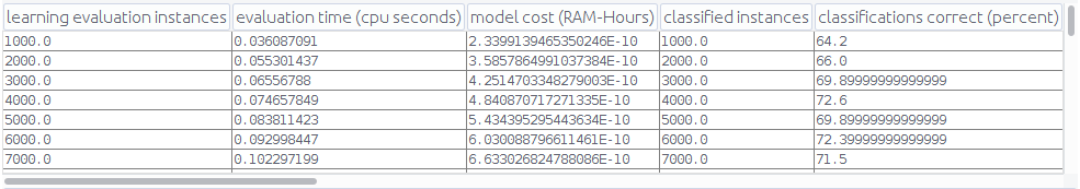
The performance of the model is periodically output, each time 10,000 examples are tested.

Connected to JobManager at Actor[akka://flink/user/jobmanager_1#-511692578] with leader session id 2639af1e-4498-4bd9-a48b-673fa21529f5.
02/20/2018 16:53:28 Job execution switched to status RUNNING.
02/20/2018 16:53:28 Source: Custom Source -> Process(1/1) switched to SCHEDULED
02/20/2018 16:53:28 Co-Flat Map(1/1) switched to SCHEDULED
02/20/2018 16:53:28 TriggerWindow(GlobalWindows(), AggregatingStateDescriptor{serializer=org.apache.flink.api.java.typeutils.runtime.kryo.KryoSerializer@463338d7, aggFunction=moa.flink.traintest.PerformanceFunction@5f2050f6}, PurgingTrigger(CountTrigger(10000)), AllWindowedStream.aggregate(AllWindowedStream.java:475)) -> Sink: Unnamed(1/1) switched to SCHEDULED
02/20/2018 16:53:28 Source: Custom Source -> Process(1/1) switched to DEPLOYING
02/20/2018 16:53:28 Co-Flat Map(1/1) switched to DEPLOYING
02/20/2018 16:53:28 TriggerWindow(GlobalWindows(), AggregatingStateDescriptor{serializer=org.apache.flink.api.java.typeutils.runtime.kryo.KryoSerializer@463338d7, aggFunction=moa.flink.traintest.PerformanceFunction@5f2050f6}, PurgingTrigger(CountTrigger(10000)), AllWindowedStream.aggregate(AllWindowedStream.java:475)) -> Sink: Unnamed(1/1) switched to DEPLOYING
02/20/2018 16:53:28 Source: Custom Source -> Process(1/1) switched to RUNNING
02/20/2018 16:53:28 TriggerWindow(GlobalWindows(), AggregatingStateDescriptor{serializer=org.apache.flink.api.java.typeutils.runtime.kryo.KryoSerializer@463338d7, aggFunction=moa.flink.traintest.PerformanceFunction@5f2050f6}, PurgingTrigger(CountTrigger(10000)), AllWindowedStream.aggregate(AllWindowedStream.java:475)) -> Sink: Unnamed(1/1) switched to RUNNING
02/20/2018 16:53:28 Co-Flat Map(1/1) switched to RUNNING
0.8958
0.9244
0.9271
0.9321
0.9342
0.9345
0.9398
0.937
0.9386
0.9415
0.9396
0.9426
0.9429
0.9427
0.9454
...

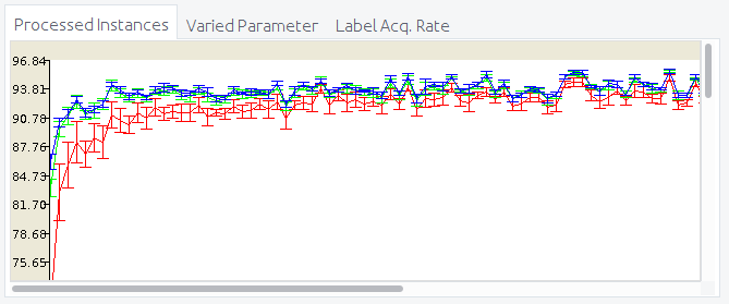
The performance of our model increase over time, as expected for on incremental machine learning algorithm!

OzaBag in Flink

Data

In this example, the data is also generated using the MOA RandomRBF generator. Many generators with the same seed run in parallel so that each classifier receive the same examples. Then to apply “online bagging (OzaBag)” each classifier put a different weight on the instance.

int k = MiscUtils.poisson(1.0, random);
if (k > 0) {
  record.setWeight(record.weight() * k);
  ht.trainOnInstance(record);
}

Model update

The model is updated every minute using a Flink ProcessFunction. In our case we save the model on disk, but it could be pushed into a web service or some other serving layer.

@Override
public void onTimer(long timestamp, OnTimerContext ctx, Collector<String> collector) throws Exception {
  // just serialize as text the model so that we can have a look at what we've got
  StringBuilder sb = new StringBuilder();
  synchronized (ht) {
    ht.getModelDescription(sb, 2);
  }
  // just collect the names of the file for logging purpose
  collector.collect("Saving model on disk, file " +
    // save the model in a file, but we could push to our online system!
    Files.write(
      Paths.get("model/FlinkMOA_" + timestamp + "_seed-" + seed + ".model"),
      sb.toString().getBytes(),
      StandardOpenOption.CREATE_NEW)
    .toString());
  // we can trigger the next event now
  timerOn = false;
}

Output with a parallelism of 4


Connected to JobManager at Actor[akka://flink/user/jobmanager_1#-425324055] with leader session id 5f617fa1-7c02-4288-b305-7d97413ee2d8.
02/21/2018 16:51:05 Job execution switched to status RUNNING.
02/21/2018 16:51:05 Source: Random RBF Source(1/4) switched to SCHEDULED
02/21/2018 16:51:05 Source: Random RBF Source(2/4) switched to SCHEDULED
...
1> HT with OzaBag seed 3 already processed 500000 examples
3> HT with OzaBag seed 2 already processed 500000 examples
...
2> HT with OzaBag seed 0 already processed 1500000 examples
4> HT with OzaBag seed 1 already processed 1500000 examples
1> HT with OzaBag seed 3 already processed 2000000 examples
3> HT with OzaBag seed 2 already processed 2000000 examples
2> Saving model on disk, file model\FlinkMOA_1519228325596_seed-0.model
4> Saving model on disk, file model\FlinkMOA_1519228325596_seed-1.model
1> Saving model on disk, file model\FlinkMOA_1519228325597_seed-3.model
3> Saving model on disk, file model\FlinkMOA_1519228325603_seed-2.model
2> HT with OzaBag seed 0 already processed 2000000 examples
1> HT with OzaBag seed 3 already processed 2500000 examples
4> HT with OzaBag seed 1 already processed 2000000 examples
...

Next step

The next step would be to assess the performance of our online bagging. It might be a bit tricky here as we need to collect all classifiers and bag them, but we need to know which one to replace in the bag when there is an update.

In the meantime you can use MOA to check the performances!

Adaptive Random Forest

Adaptive Random Forest (ARF for short) [1] is an adaptation of the original Random Forest algorithm [2], which has been successfully applied to a multitude of machine learning tasks. In layman’s terms the original Random Forest algorithm is an ensemble of decision trees, which are trained using bagging and where the node splits are limited to a random subset of the original set of features. The “Adaptive” part of ARF comes from its mechanisms to adapt to different kinds of concept drifts, given the same hyper-parameters.

Specifically, the 3 most important aspects of the ARF algorithm are:

  1. It adds diversity through resampling (“bagging”);
  2. It adds diversity through randomly selecting subsets of features for node splits (See moa.classifiers.trees.ARFHoeffdingTree.java);
  3. It has one drift and warning detector per base tree, which cause selective resets in response to drifts. It also allows training background trees, which start training if a warning is detected and replace the active tree if the warning escalates to a drift.

ARF was designed to be “embarrassingly” parallel, in other words, there are no dependencies between trees. This allowed an easy parallel implementation of the algorithm in MOA (see parameter numberOfJobs).

Parameters

Currently, the ARF is configurable using the following parameters in MOA:

  • treeLearner (-l). ARFHoffedingTree is the base tree learner, the important default value is the grace period = 50 (this causes trees to start splitting earlier)
  • ensembleSize (-s). Ensemble size from 10 to 100 (default is 10, but the model tends to improves as more trees are added)
  • mFeaturesMode (-o). Features per subset mode = sqrt(M)+1, which corresponds to sqrt(M) + 1 that is the default for Random Forest algorithms, still it is an hyper-parameter and can be tuned for better results (this can be controlled by changing the mFeaturesMode).
  • mFeaturesPerTreeSize (-m). This controls the size features subsets based on the kFeaturesMode. For example, if mFeaturesMode = sqrt(M)+1 then this parameter is ignored, but if mFeaturesMode = “Specified m” then the value defined in for -m is considered.
  • lambda (-a). Defaults to the same as leveraging bagging, i.e., lambda = 6.
  • numberOfJobs (-j). Defines the number of threads used to train the ensemble, default is 1.
  • driftDetectionMethod (-x). Best results tend to be obtained by using ADWINChangeDetector, the default deltaAdwin (ADWIN parameter) is 0.00001. Still other drift detection methods can be easily configured and used, such as PageHinkley, DDM, EDDM, etc.
  • warningDetectionMethod (-p). This parameter controls the warning detector, such that whenever it triggers a background tree starts training along with the tree where the warning was triggered. It is important that whatever parameters are used in here, that this is consistent with the driftDetectionMethod, i.e., the warning should always trigger before the drift to guarantee the overall algorithm’s expected behavior. The default values are ADWINChangeDetector with deltaAdwin = 0.0001, notice that this is 10x greater than the default deltaAdwin for the driftDetectionMethod.
  • disableWeightedVote (-w). If this is set, then predictions will be based on majority vote instead of weighted votes. The default is to use weighted votes, thus this is not set.
  • disableDriftDetection (-u). This controls if drift detection is used, when set there will be no drift or warning detection as well as background learners are not created, independently of any other parameters. The default is to use drift detection, thus this is not set.
  • disableBackgroundLearner (-q). When set the background learner is not used as well as the warning detector is ignored (there are no checks for warning). The default is to use background learners, thus this is not set.

Comparing against the Adaptive Random Forest

A practical and simple way to compare against Adaptive Random Forest is to compare classification performance in terms of Accuracy/Kappa M and Kappa T using the traditional immediate setting, where  the true label is presented right after the instance has been used for testing, or the delayed setting, where there is a delay between the time an instance is presented and its true label becomes available.

In this post we present some practical and simple ways to compare against ARF, for a thorough comparison against other state-of-the-art ensemble classifiers and thorough discussion of other aspects of ARF (e.g. weighted vote) please refer to publication [1].

Evaluator task Adaptive Random Forest

In [1] the evaluator tasks used were EvaluatePrequential, EvaluatePrequentialCV, EvaluatePrequentialDelayed and EvaluatePrequentialCV. CV stands for Cross-Validation and more details about it can be found in [3]. In this example we are only going to use EvaluatePrequential as CV versions take longer to run, however one can easily change from EvaluatePrequential to EvaluatePrequentialCV and obtain the CV results or EvaluatePrequentialDelayed (and EvaluatePrequentialDelayedCV) to obtain delayed labeling results.

ARF fast and moderate

In the original paper, there are 2 main configurations that should be useful to compare against future algorithms, they were identified as ARF_{moderate} and ARF_{fast}. Basically ARF_{moderate} is the standard configuration (described in the default parameters values above) and ARF_{fast} increases the deltaAdwin (e.g. the default drift detector is ADWINChangeDetector for -x and -p) for both warning and drift detection causing more detections.

To test AdaptiveRandomForest in either delayed or immediate setting execute the latest MOA jar.
You can copy and paste the following commands in the interface (right click the configuration text edit and select “Enter configuration”).

Airlines dataset, ARF_{moderate} (default configuration) with 10 trees.
EvaluatePrequential -l (meta.AdaptiveRandomForest) -s (ArffFileStream -f airlines.arff) -e BasicClassificationPerformanceEvaluator -f 54000

Airlines dataset, ARF_{fast} (detect drifts earlier and yield false positives) with 10 trees.
EvaluatePrequential -l (meta.AdaptiveRandomForest -x (ADWINChangeDetector -a 0.001) -p (ADWINChangeDetector -a 0.01)) -s (ArffFileStream -f airlines.arff) -e BasicClassificationPerformanceEvaluator -f 54000

Airlines dataset, LeveragingBagging with 10 trees
EvaluatePrequential -l meta.LeveragingBag -s (ArffFileStream -f airlines.arff) -e BasicClassificationPerformanceEvaluator -f 54000

Explanation: All these commands executes EvaluatePrequential with BasicClassificationPerformanceEvaluator (this is equivalent to InterleavedTestThenTrain) on the airlines dataset (-f airlines.arff). The tree commands use 10 trees (-s 10 is implicit in all three cases). ARF also uses m = sqrt(total features) + 1 and the difference between ARF_{moderate} and ARF_{fast} remains on the detectors parameters. Make sure to extract the airlines.arff dataset, and setting -f to its location, before executing the command. The airlines and others datasets are available in here: https://github.com/hmgomes/AdaptiveRandomForest.

[1] Heitor Murilo Gomes, Albert Bifet, Jesse Read, Jean Paul Barddal, Fabricio Enembreck, Bernhard Pfharinger, Geoff Holmes, Talel Abdessalem. Adaptive random forests for evolving data stream classification. In Machine Learning, DOI: 10.1007/s10994-017-5642-8, Springer, 2017.

This can be downloaded from Springer: https://rdcu.be/tsdi
The pre-print is also available in here: Adaptive Random Forest pre-print

[2] Breiman, Leo. Random forests.Machine Learning 45.1, 5-32, 2001.

[3] Albert Bifet, Gianmarco De Francisci Morales, Jesse Read, Geoff Holmes, Bernhard Pfahringer: Efficient Online Evaluation of Big Data Stream Classifiers. KDD 2015: 59-68

New Release of MOA 17.06

We’ve made a new release of MOA 17.06

The new features of this release are:

  • SAMKnn:
    • Viktor Losing, Barbara Hammer, Heiko Wersing: KNN Classifier with Self Adjusting Memory for Heterogeneous Concept Drift. ICDM 2016: 291-300
  • Adaptive Random Forest:
    • Heitor Murilo Gomes, Albert Bifet, Jesse Read, Jean Paul Barddal, Fabricio Enembreck, Bernhard Pfharinger, Geoff Holmes, Talel Abdessalem. Adaptive random forests for evolving data stream classification. In Machine Learning, Springer, 2017.
  • Blast:
    • Jan N. van Rijn, Geoffrey Holmes, Bernhard Pfahringer, Joaquin Vanschoren: Having a Blast: Meta-Learning and Heterogeneous Ensembles for Data Streams. ICDM 2015: 1003-1008
  • Prequential AUC:
    • Dariusz Brzezinski, Jerzy Stefanowski: Prequential AUC: properties of the area under the ROC curve for data streams with concept drift. Knowl. Inf. Syst. 52(2): 531-562 (2017)
  • D-Stream:
    • Yixin Chen, Li Tu: Density-based clustering for real-time stream data. KDD 2007: 133-142
  • IADEM:
    • Isvani Inocencio Frías Blanco, José del Campo-Ávila, Gonzalo Ramos-Jiménez, André Carvalho, Agustín Alejandro Ortiz Díaz, Rafael Morales Bueno: Online adaptive decision trees based on concentration inequalities. Knowl.-Based Syst. 104: 179-194 (2016)
  • RCD Classifier:
    • Gonçalves Jr, Paulo Mauricio, and Roberto Souto Maior De Barros: RCD: A recurring concept drift framework. Pattern Recognition Letters 34.9 (2013): 1018-1025.
  • ADAGrad:
    • John C. Duchi, Elad Hazan, Yoram Singer: Adaptive Subgradient Methods for Online Learning and Stochastic Optimization. Journal of Machine Learning Research 12: 2121-2159 (2011)
  • Dynamic Weighted Majority:
    • J. Zico Kolter, Marcus A. Maloof: Dynamic Weighted Majority: An Ensemble Method for Drifting Concepts. Journal of Machine Learning Research 8: 2755-2790 (2007)
  • StepD:
    • Kyosuke Nishida, Koichiro Yamauchi: Detecting Concept Drift Using Statistical Testing. Discovery Science 2007: 264-269
  • LearnNSE:
    • Ryan Elwell, Robi Polikar: Incremental Learning of Concept Drift in Nonstationary Environments. IEEE Trans. Neural Networks 22(10): 1517-1531 (2011)
  • ASSETS Generator:
    • Jean Paul Barddal, Heitor Murilo Gomes, Fabrício Enembreck, Bernhard Pfahringer, Albert Bifet: On Dynamic Feature Weighting for Feature Drifting Data Streams. ECML/PKDD (2) 2016: 129-144
  • SineGenerator and MixedGenerator:
    • Joao Gama, Pedro Medas, Gladys Castillo, Pedro Pereira Rodrigues: Learning with Drift Detection. SBIA 2004: 286-295
  • AMRulesMultiLabelLearnerSemiSuper (Semi-supervised Multi-target regressor):
    • Ricardo Sousa, Joao Gama: Online Semi-supervised Learning for Multi-target Regression in Data Streams Using AMRules. IDA 2016: 123-133
  • AMRulesMultiLabelClassifier (Multi-label classifier):
    • Ricardo Sousa, Joao Gama: Online Multi-label Classification with Adaptive Model Rules. CAEPIA 2016: 58-67
  • WeightedMajorityFeatureRanking, MeritFeatureRanking and BasicFeatureRanking (Feature ranking methods)
    • Joao Duarte, Joao Gama: Feature ranking in hoeffding algorithms for regression. SAC 2017: 836-841
  • AMRulesMultiTargetRegressor (Multi-target regressor):
    • Joao Duarte, Joao Gama, Albert Bifet: Adaptive Model Rules From High-Speed Data Streams. TKDD 10(3): 30:1-30:22 (2016)

You can find the download link for this release on the MOA homepage:

MOA Machine Learning for Streams

Cheers,

The MOA Team

New Release of MOA 16.04

We’ve made a new release of MOA 16.04.

The new features of this release are:

  • BICO: BIRCH Meets Coresets for k-Means Clustering.
    • Hendrik Fichtenberger, Marc Gillé, Melanie Schmidt,
      Chris Schwiegelshohn, Christian Sohler: ESA 2013: 481-492 (2013)
      https://ls2-www.cs.tu-dortmund.de/bico/
  • Updates:
    • MultiLabel and MultiTarget methods

There are these important changes after MOA 2015.11 release:

  • Use Examples instead of Instances to be able to deal easily with unstructured data
  • Use Apache Samoa instances instead of WEKA instances
  • Use the javacliparser library

You find the download link for this release on the MOA homepage:

MOA Machine Learning for Streams

Cheers,

The MOA Team