by Yongheng Ma, Heitor Murilo Gomes,  Albert Bifet on December 18, 2020 using MOA 2020.12.

1. Getting started

This tutorial shows how to use MOA newest module “Feature Analysis” to visualize features and feature importance of a data stream. This kind of analysis allows data scientists and researchers to quickly identify temporal dependencies and fluctuations on the feature importances, which may indicate feature drifts.

This tutorial is divided into 3 parts. First, we introduce the GUI (graphical user interface) for the “Feature Analysis” module. Then we show how to use the VisualizeFeatures tab. Finally, we explain how to use the FeatureImportance tab.

Disclaimer

• This tutorial was originally developed for MOA Release 2020.12 (available here: here).
• We assume you are familiar with what is MOA and the MOA GUI. If that is not the case, you probably should check this tutorial first
• We assume you are familiar with what is feature importance. In summary, it is a way to quantify the importance of a feature to a given model. If you want to know more about it, specially in a streaming setting, then please refer to [1].
• Feature importances can be obtained in MOA by using the meta-classifier moa.learner.analysis.classifierWithFeatureImportance. This will output a report of the feature importances in a CSV format. In this tutorial, we show how to accomplish that using the GUI, so that the user can visualize them on MOA.

Requirements

• MOA Release 2020.12 or later (available here: here).

2. The Feature Analysis GUI

After launching MOA, select the “Feature Analysis” from the list, (1) in the figure below, you should see the following GUI.

The elements in the GUI:

(2) The VisualizeFeature tab includes information about the features such as current relation, all attributes, selected attribute and its’ statistical information, as well as different kinds of graphs. Before loading the data stream, all content is empty.

(3) The FeatureImportance tab allows the execution of Feature Importance algorithms (illustrated in detail later in this tutorial).

3. VisualizeFeatures tab

This tab allows the visualization of features “over time.”

3.1 Loading a data stream from an ARFF file

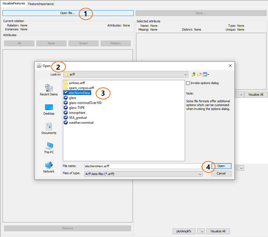
The “Open file…” button, (1) shows the open file dialog (2), where the user can choose an ARFF file, (3) and (4).

After loading the data, a variety of functions can be used in the VisualizeFeatures tab, as shown below:

(1) The current relation information (i.e. name of the dataset) including relation name, attribute count and instance number;

(2) It shows all the features names, the checkboxes can be used to select features for removal;

(3) Remove button is used to remove one or multiple features;

(4) After deleting one or multiple attributes values, the save button can be used to save the transformed dataset.

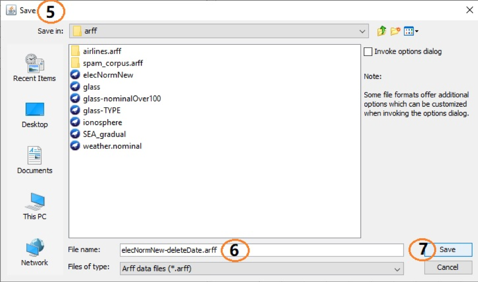
(5) When user clicks (4), a save dialog will show up.

(6) The name of the new dataset.

(7) Save button .

(8) When user selects one or multiple attributes from (2), (8) displays the summary information of the last attribute selected, such as missing values, distinct, unique, min, max, mean and stdDev.

(9) By default, (9) shows the histogram of the class attribute. When other attribute is selected from the dropdown list, it displays the corresponding histogram.

(10) Button “Visualize All” for histograms.

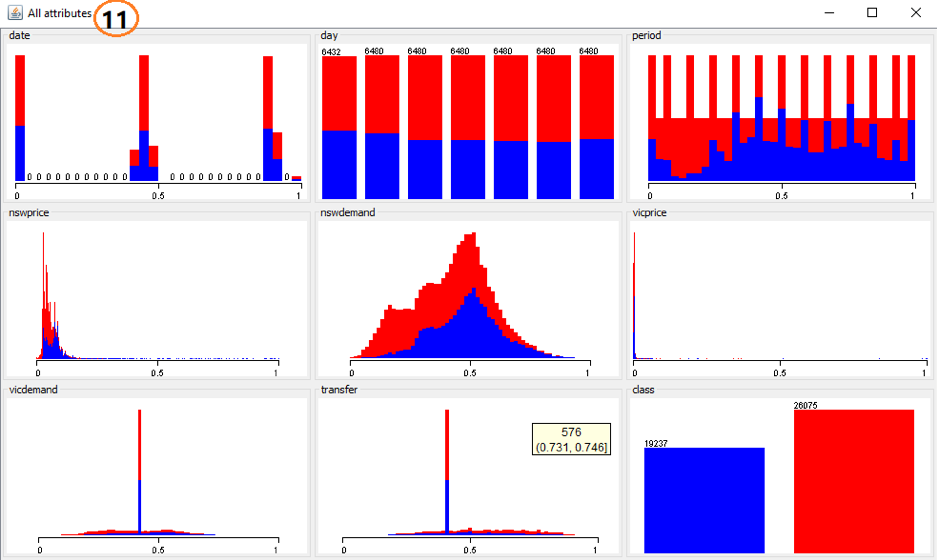
(11) The view after clicking on (10) displays the histograms for every feature.

(12) The selected feature’s line graph or scatter diagram. For nominal feature, only scatter diagram are presented; for numeric features, both the line graph and scatter diagram are available. The details of the (12) are illustrated as follows.

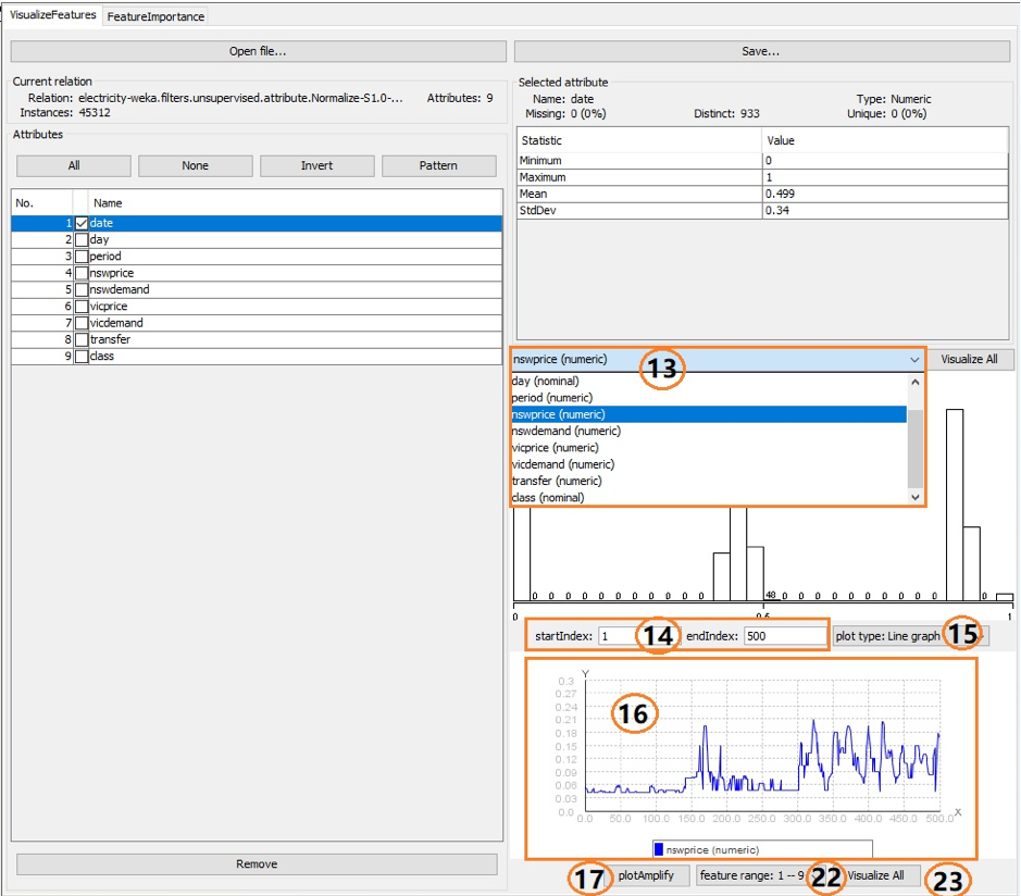
(13) User chooses an attribute from the attributes dropdown list and the values will be shown as histogram, line graph or scatter diagram.

(14) “startIndex” and “endIndex” determines the instance index range displayed in a line graph or a scatter diagram. By default, the startIndex is 1, the endIndex is 500. If the number of instances is less than 500, then “endIndex” = number of instances.

(15) Line graphs and scatter diagrams are available for numerical features, while nominal features can only be displayed with scatter diagrams.

(16) It displays the line graph or scatter diagram according to the selected feature, instance range and plot type.

(17) “plotAmplify” button pop up a full screen plot in (16) so that the user can observe the graph more clearly. The amplified graph provides several convenient tools.

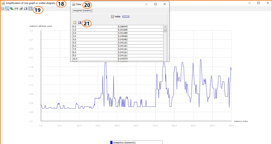
(18) The amplification of a line graph or a scatter diagram.

(19) The tools bar provides seven options. If the user selects (19), then a pop up data window will display the feature values as in (20).

(20) The pop up data window .

(21) The “copy data to clipboard” and “save data into ASCII file”.

(22) This droplist provides feature range choices which represent the specific features to be shown as graphs when the user clicks button Visualize All (23). For example, if a dataset has 23 features, then the droplist will have 3 choices “feature range: 1 — 9”, “feature range: 10 — 18”, “feature range: 19 — 23”.

(23) If a user selects “feature range: 1 — 9” in (22) and clicks the button Visualize All, MOA will pop up a window to show 9 graphs as (24).

(24) It shows graphs according to (22) and (15). For nominal features, whether plot type is line graph or scatter diagram, (24) only shows scatter diagrams. For the numeric feature, plot type decides the plot type displayed in (24).

4. FeatureImportance tab

Feature importance is a way to quantify the relevance of a feature to a specific model [1]. For example, the impact of the features in a Random Forest classification model can be estimated through several metrics, such as COVERAGE, MDI and MDA. More details about the available algorithms can be found in section 4.3.

The precondition for using the functions in this tab is to load the data stream first in the “VisualizeFeatures” tab. In other words, before a user clicks the run button, the data stream should have been loaded, otherwise an error will be displayed “Please open data stream file from VisualizerFeatures tab first!”

4.1 Configuring the parameters

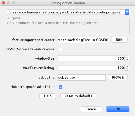
When a user clicks the configure button the following GUI will be displayed. Details about how to configure the “FeatureImportanceLearner” are presented in section 4.3, the other elements of the GUI are commented below:

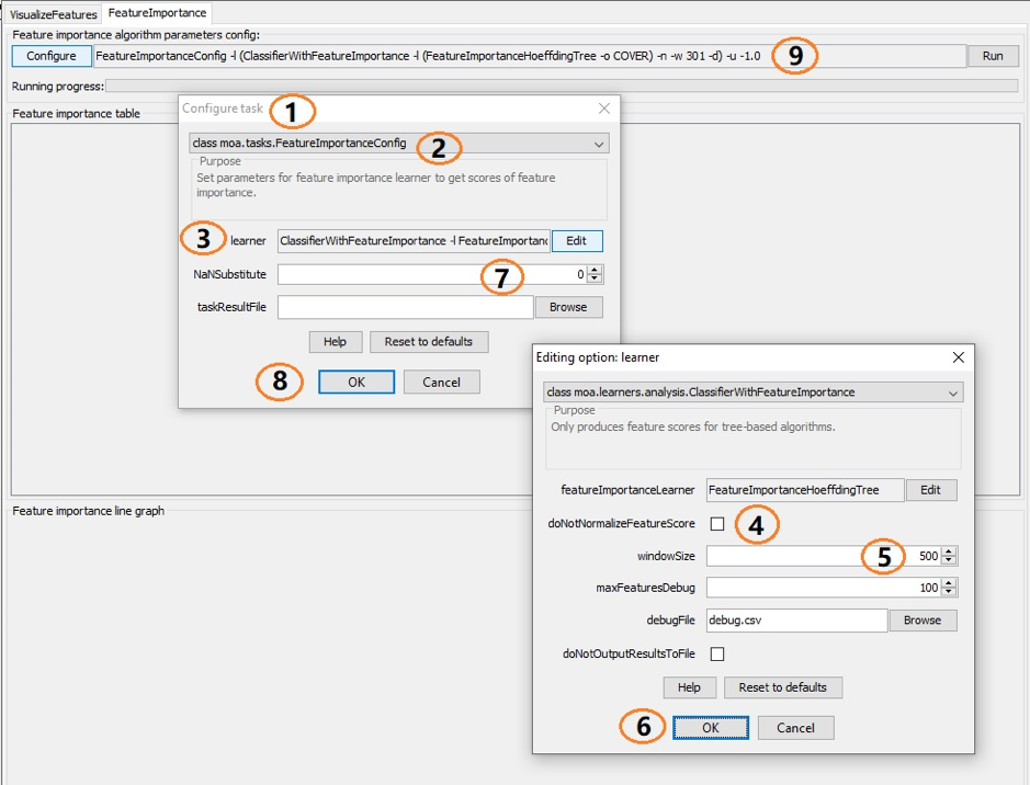
(1) Configure task menu

(2) Class “tasks.FeatureImportanceConfig” option which is the first critical option

(3) The edit button brings the configure learner related options. The only option for the the learner is “moa.learner.analysis.classifierWithFeatureImportance”

(4) “doNotNormalizeFeatureScore” decides whether the feature importance is normalized. By default, this option is not set and the results are normalized

(5) “WindowSize” is the number of instances seen before inspecting the feature importance again. By default, the windowSize parameter is 500

(6) The feature importances can also be output to a file, then the options “maxFeaturesDebug”, “debugFile”, “doNotOutputResultsToFile”, should be set

(7) The scores of feature importance may be values like 4686.86537331929, 0.053471126481504741, 0.0, 1.0, NaN. NaN values can be replaced by a double value so that it can be shown in the line graph. By default, the “NaNSubstitute” parameter is 0

(8) Confirm the selected configurations

(9) The configuration is composed as a command line (CLI) which can be copied to the clipboard and used in other tabs or saved for fast configuration

4.2 Running the model

After configuring the options, the following GUI will be displayed. The elements numbered in the GUI are explained below:

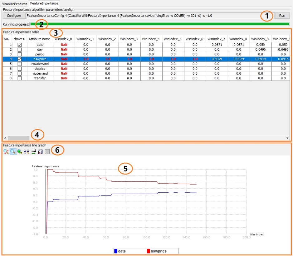
(1) The “Run” button. If the configuration is changed, it can be run again, but previous feature importances will be lost (unless they are saved to a file using “debugFile”).

(2) After clicking the “Run” button, the model will produce scores of the feature importance and the progress bar will start updating.

(3) The feature importance table is used to show the feature importance of each feature in different windows. For example, the scores of feature “date” in the screen shot are “NaN, 0.0, 0.0, 0.0, 0.0, 0.0, 0.0, 0.0671, 0.0671, 0.059, 0.059, …” in the sequential window index. Windows count is equal the floor(numInstances/windowSize). For example, numInstances is 205 and windowSize is 20, then floor(numInstances / windowSize) is 10 and the window index starts from 0.

(4) If there are many winIndexs, a user can scroll the horizontal bar to see all the scores.

(5) User selects features from the feature importance table, the corresponding line graphs of the features’ scores will be shown. User deselects features from the feature importance table, the corresponding line graphs will disappear. By default, the plot shows the first feature’s scores if a user selects none of the features.

(6) The plot tools bar shows here. For example, if user clicks the tool to the right, the data window pop up will appear to show feature scores which can be saved as an ASCII file or copied to the clipboard to be analyzed furthermore.

4.3 The feature importance API

The feature importance API was designed to allow extensibility (to add new methods) and compatibility (to not interfere with existing algorithms). Currently, the implementation is based on the algorithms presented in [1], so the focus is on Hoeffding Trees [2] and their subclasses, and ensembles of Hoeffding Trees. A breakdown of the classes that compose the feature importance API is shown below:

• ClassifierWithFeatureImportance: This meta-classifier serves the purpose of executing a classifier also capable of outputting feature importances. It can be used from the Classification tab as well as part of the Feature Analysis tab (as described in this tutorial).
• FeatureImportanceClassifier: This interface defines the methods to be implemented on a Classifier to allow it to produce feature importances. Developers and researchers looking to add new algorithms to produce Feature Importances must implement this class.
• FeatureImportanceHoeffdingTree: This class uses the HoeffdingTree structure (composition) to produce feature importances. This class does not interfere with the training algorithm of the underlying HoeffdingTree model. Any subclass of the HoeffdingTree class can be set as the treeLearnerOption, including the Hoeffding Adaptive Tree (HAT) [3].
• FeatureImportanceHoeffdingTreeEnsemble: This class enables the generation of feature importances from ensembles of HoeffdingTree models (and its subclasses), such as the Adaptive Random Forest (ARF) [4] and Streaming Random Patches (SRP) [5]. This class does not interfere with the training algorithm of the underlying ensemble model. The base learner of the ensemble model must be either a HoeffdingTree or one of its subclasses.

Flexibility and compatibility come at the price of a slightly intricate GUI.  The best way to understand it is through examples. We explain below how to execute a Hoeffding Adaptive Tree to obtain the MDI feature importance and then proceed to do the same for Adaptive Random Forest (ARF) using the COVER feature importance.

4.3.1 Hoeffding Adaptive Tree using MDI

(1) Choose the “configure” button in the Feature Importance tab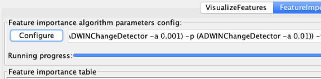

(2) Edit the “learner” option(3) Edit the “featureImportanceLearner”

(4) Make sure the “FeatureImportanceHoeffdingTree” is selected in the dropdown

(5) Edit the “treeLearner” to select the “HoeffdingAdaptiveTree”

(6) Make sure “MDI” is selected in the dropdown for “featureImportance”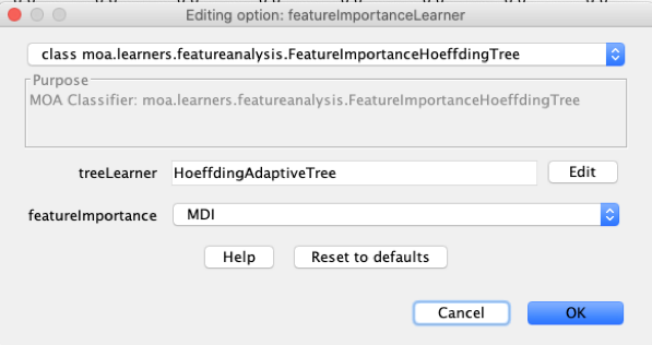

The following command line will be generated:

“FeatureImportanceConfig -l (ClassifierWithFeatureImportance -l (FeatureImportanceHoeffdingTree -l HoeffdingAdaptiveTree) -d)”

4.3.2 Adaptive Random Forest using COVER

(7) Follow steps (1) to (3) to reach the “featureImportanceLearner” configuration.

(8) Select “FeatureImportanceHoeffdingTreeEnsemble” in the dropdown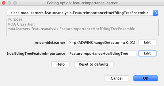

(9) Edit the “ensembleLearner” to select the “AdaptiveRandomForest” algorithm. Tip: by default ARF uses 100 trees, for a preliminary test you might want to set it to 10.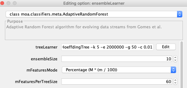  

(10) Edit the “hoeffdingTreeFeatureImportance” and then select “COVER” in the dropdown for “featureImportance”.

(11) IMPORTANT: Notice that the “treeLearner” option of the “featureImportance”, when configured from within the “FeatureImportanceHoeffdingTreeEnsemble” has no effect. Internally, it will be overridden by the Hoeffding Tree subclass object from the ensemble model.

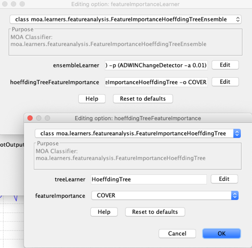
The following command line will be generated:

FeatureImportanceConfig -l (ClassifierWithFeatureImportance -l (FeatureImportanceHoeffdingTreeEnsemble -l (meta.AdaptiveRandomForest -l (ARFHoeffdingTree -k 5 -e 2000000 -g 50 -c 0.01) -s 10 -x (ADWINChangeDetector -a 0.001) -p (ADWINChangeDetector -a 0.01)) -t (FeatureImportanceHoeffdingTree -o COVER)) -d)

References

[1] Gomes, H. M., de Mello, R. F., Pfahringer, B., & Bifet, A. (2019, December). Feature Scoring using Tree-Based Ensembles for Evolving Data Streams. In 2019 IEEE International Conference on Big Data (Big Data) (pp. 761-769). IEEE.

[2] Domingos, Pedro, and Geoff Hulten. “Mining high-speed data streams.” In Proceedings of the sixth ACM SIGKDD international conference on Knowledge discovery and data mining, pp. 71-80. 2000.

[3] Bifet, Albert, and Ricard Gavaldà. “Adaptive learning from evolving data streams.” In International Symposium on Intelligent Data Analysis, pp. 249-260. Springer, Berlin, Heidelberg, 2009.

[4] Gomes, Heitor M., Albert Bifet, Jesse Read, Jean Paul Barddal, Fabrício Enembreck, Bernhard Pfahringer, Geoff Holmes, and Talel Abdessalem. “Adaptive random forests for evolving data stream classification.” Machine Learning 106, no. 9-10 (2017): 1469-1495.

[5] Gomes, Heitor Murilo, Jesse Read, and Albert Bifet. “Streaming random patches for evolving data stream classification.” In 2019 IEEE International Conference on Data Mining (ICDM), pp. 240-249. IEEE, 2019.