by Peter Reutemann, Albert Bifet on October 28, 2017.
Getting Started
This tutorial is a basic introduction to use ADAMS and MOA.
https://adams.cms.waikato.ac.nz/
WEKA and MOA are powerful tools to perform data mining analysis tasks. Usually, in real applications and professional settings, the data mining processes are complex and consist of several steps. These steps can be seen as a workflow. Instead of implementing a program in JAVA, a professional data miner will build a solution using a workflow, so that it will be much easier to maintain for non-programmer users.
The Advanced Data mining And Machine learning System (ADAMS) is a novel, flexible workflow engine aimed at quickly building and maintaining real-world, complex knowledge workflows.
The core of ADAMS is the workflow engine, which follows the philosophy of less is more. Instead of letting the user place operators (or actors in ADAMS terms) on a canvas and then manually connect inputs and outputs, ADAMS uses a tree-like structure. This structure and the control actors define how the data is flowing in the workflow, no explicit connections necessary. The tree-like structure stems from the internal object representation and the nesting of sub-actors within actor-handlers.
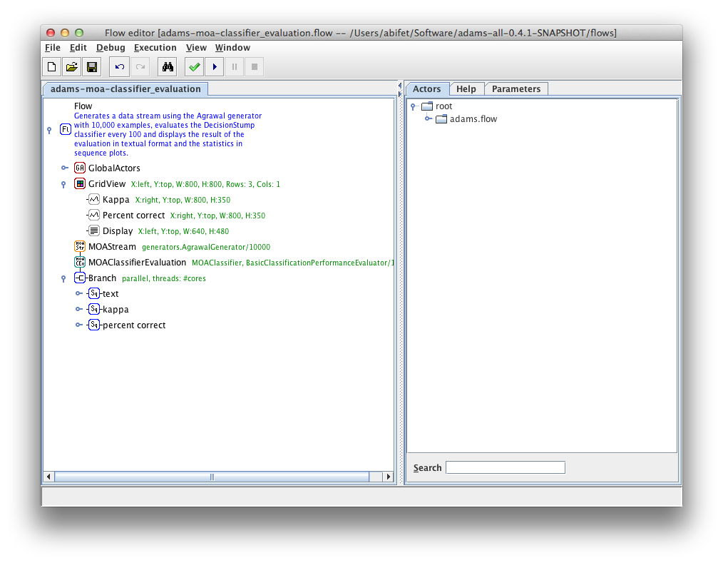
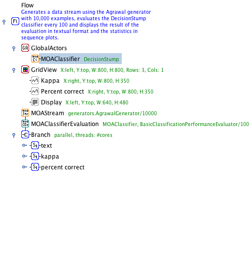
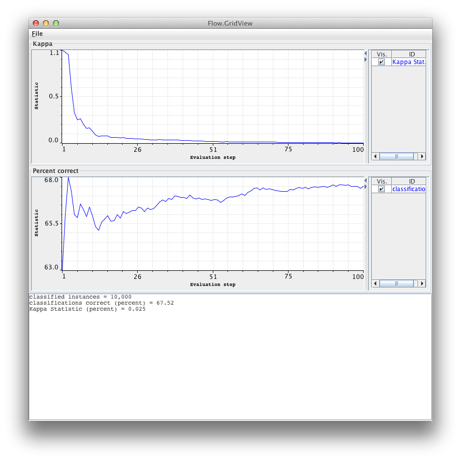
We suppose that ADAMS is installed in your system. Start the Flow Editor and load the adams-moa-classifier-evaluation flow. Run the flow. Note that:
- Kappa statistic is a measure of agreement of a classifier with a ran- dom one. If Kappa statistic is zero, the classifier is performing as a random one, and if it is equal to one, then it is not random at all.
- A decision stump is a decision tree with only one split node.
Exercise 1 Explain what this workflow does. Discuss why accuracy is increasing and kappa statistic is decreasing. What happens if you replace the decision stump by a Hoeffding Tree?
Classification using ADAMS
We start comparing the accuracy of two classifiers. First, we explain briefly two different data stream evaluations.
Data streams Evaluation
The most significant requirements for a data stream setting are the following:
- Requirement 1 Process an example at a time, and inspect it only once (at most)
- Requirement 2 Use a limited amount of memory
- Requirement 3 Work in a limited amount of time
- Requirement 4 Be ready to predict at any time
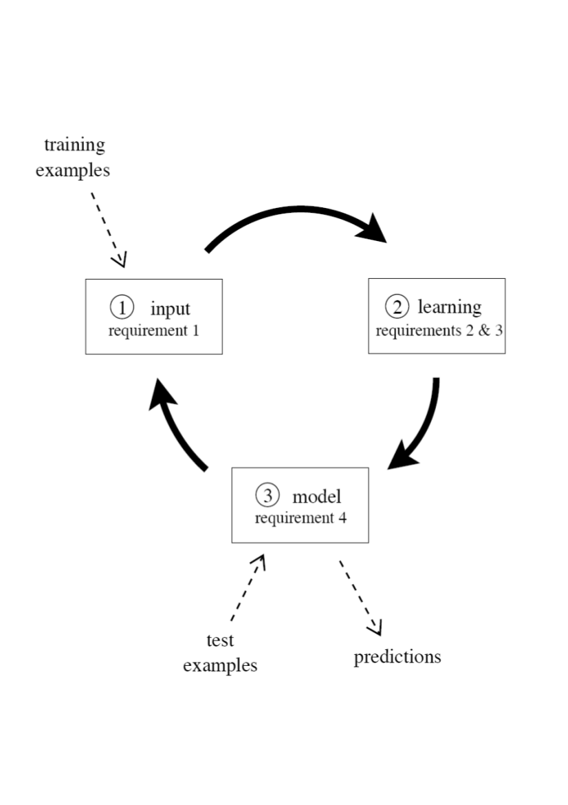
This figure illustrates the typical use of a data stream classification algorithm, and how the requirements fit in a repeating cycle:
- The algorithm is passed the next available example from the stream (requirement 1).
- The algorithm processes the example, updating its data structures. It does so without exceeding the memory bounds set on it (requirement 2), and as quickly as possible (requirement 3).
- The algorithm is ready to accept the next example. On request it is able to predict the class of unseen examples (requirement 4).
In traditional batch learning the problem of limited data is overcome by analyzing and averaging multiple models produced with different random arrangements of training and test data. In the stream setting the problem of (effectively) unlimited data poses different challenges. One solution involves taking snapshots at different times during the induction of a model to see how much the model improves.
When considering what procedure to use in the data stream setting, one of the unique concerns is how to build a picture of accuracy over time. Two main approaches arise:
- Holdout: When traditional batch learning reaches a scale where cross-validation is too time consuming, it is often accepted to instead measure performance on a single holdout set. This is most useful when the division between train and test sets have been pre-defined, so that results from different studies can be directly compared.
- Interleaved Test-Then-Train or Prequential: Each individual example can be used to test the model before it is used for training, and from this the accuracy can be incrementally updated. When intentionally performed in this order, the model is always being tested on examples it has not seen. This scheme has the advantage that no holdout set is needed for testing, making maximum use of the available data. It also ensures a smooth plot of accuracy over time, as each individual example will become increasingly less significant to the overall average.
Holdout evaluation gives a more accurate estimation of the accuracy of the classifier on more recent data. However, it requires recent test data that it is difficult to obtain for real datasets. Gama et al. propose to use a forgetting mechanism for estimating holdout accuracy using prequential accuracy: a sliding window of size w with the most recent observations, or fading factors that weigh observations using a decay factor 


As data stream classification is a relatively new field, such evaluation practices are not nearly as well researched and established as they are in the traditional batch setting.
Exercises
To familiarize yourself with the functions discussed so far, please do the following two exercises, loading and modifying the adams-moa-compare-classifiers flow.
Exercise 2. Compare the accuracy of the Hoeffding Tree with the Naive Bayes classifier, for a RandomTreeGenerator stream of 10,000 instances using Interleaved Test-Then-Train evaluation.
Exercise 3. Compare and discuss the accuracy for the same stream of the previous exercise using two different evaluations with a Hoeffding Tree:
- Interleaved Test Then Train
- Prequential with a sliding window of 100 instances.
Drift Stream Generators
MOA streams are build using generators, reading ARFF files, joining several streams, or filtering streams. MOA streams generators allow to simulate potentially infinite sequence of data.
Two streams evolving on time are:
- Rotating Hyperplane
- Random RBF Generator
To model concept drift we only have to set up the drift parameter of the stream.
Exercises
Exercise 4. Compare the accuracy of the Hoeffding Tree with the Naive Bayes classifier, for a RandomRBFGenerator stream of 50,000 instances with speed change of 0,001 using Interleaved Test-Then-Train evaluation.
Exercise 5. Compare the accuracy for the same stream of the previous exercise using three different classifiers:
- Hoeffding Tree with Majority Class at the leaves
- Hoeffding Adaptive Tree
- OzaBagAdwin with 10 HoeffdingTree