by Frederic Stahl on October 28, 2017 using MOA 2017.06.

This tutorial is a basic introduction on how to perform clustering using MOA.

Task 1: Getting Started

MOA provides implementations of several clustering streaming algorithms. For experimental purposes MOA also provides an evolving artificial data stream generator where the ground truth is known. It is also possible to stream in data from a file in the ARFF format (http://www.cs.waikato. ac.nz/ml/weka/arff.html). In this tutorial we are going to use the artificial stream generator.

GUI for clustering task configuration

After starting MOA, if you select the Clustering tab (element 1 in the figure below), you should see the following GUI.

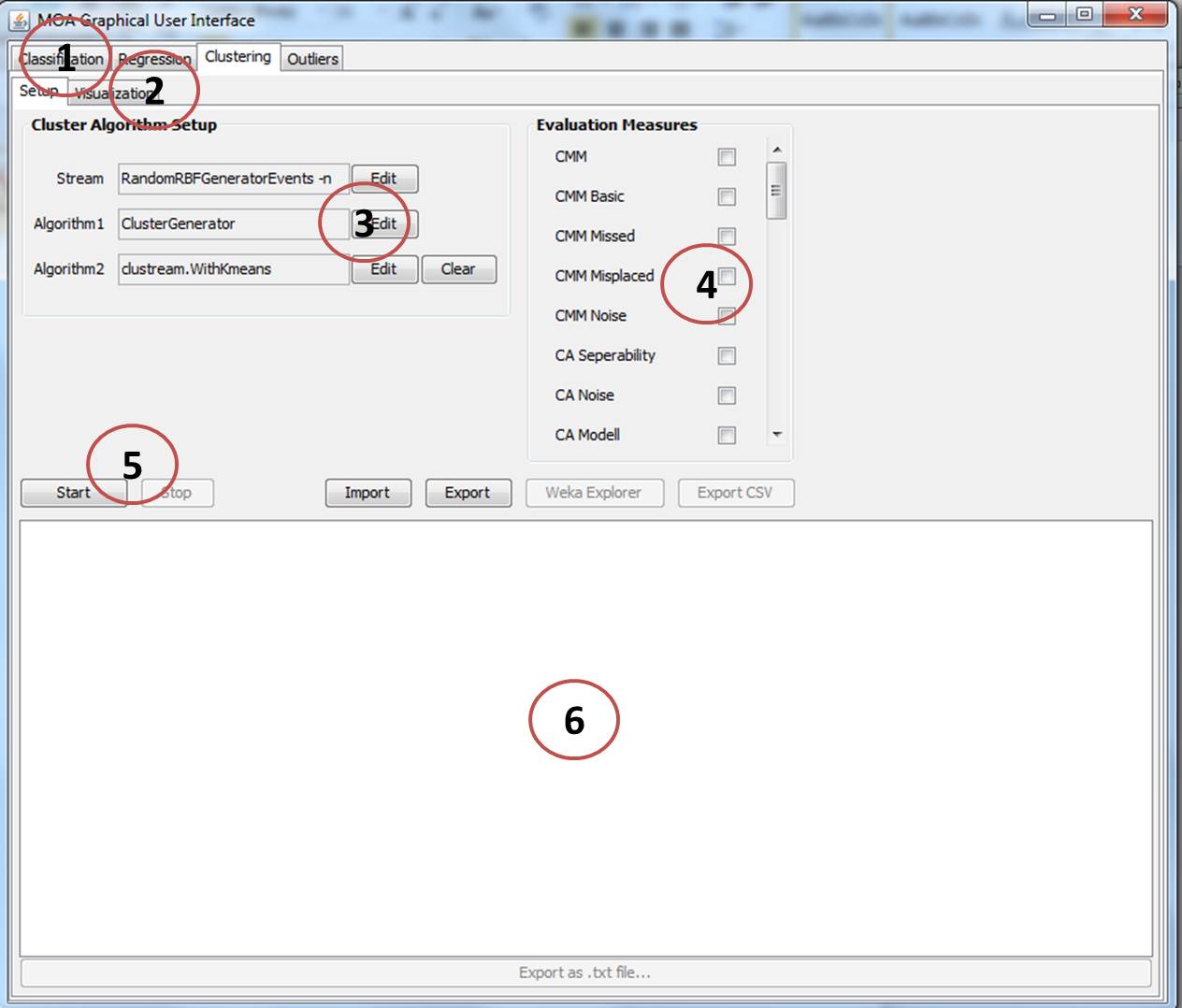
The elements numbered in the GUI are explained below:

• Element 1 There are several tabs, classification, regression, clustering, outliers and others. Here the clustering tab is selected.
• Element 2 The Clustering GUI is divided into two parts, “setup” and “visualisation”. These two parts can be selected through the two tabs in this element. In Figure 1, “Setup” is selected.
• Element 3 Here you can select and configure a data stream and two clustering algorithms that be executed and compared in real time in MOA.
• Element 4 Here you can select various evaluation metrics that can be used for evaluating the clustering algorithms. The here selected metrics will also be available in the “visualisation” part of the clustering GUI.
• Element 5 With these buttons you can start or stop the clustering task.
• Element 6 Shows the command line output.

GUI for clustering task visualisation

If you select the visualisation part in Element 2 of the clustering GUI (and click on the “Start” button), then you should see something like this:

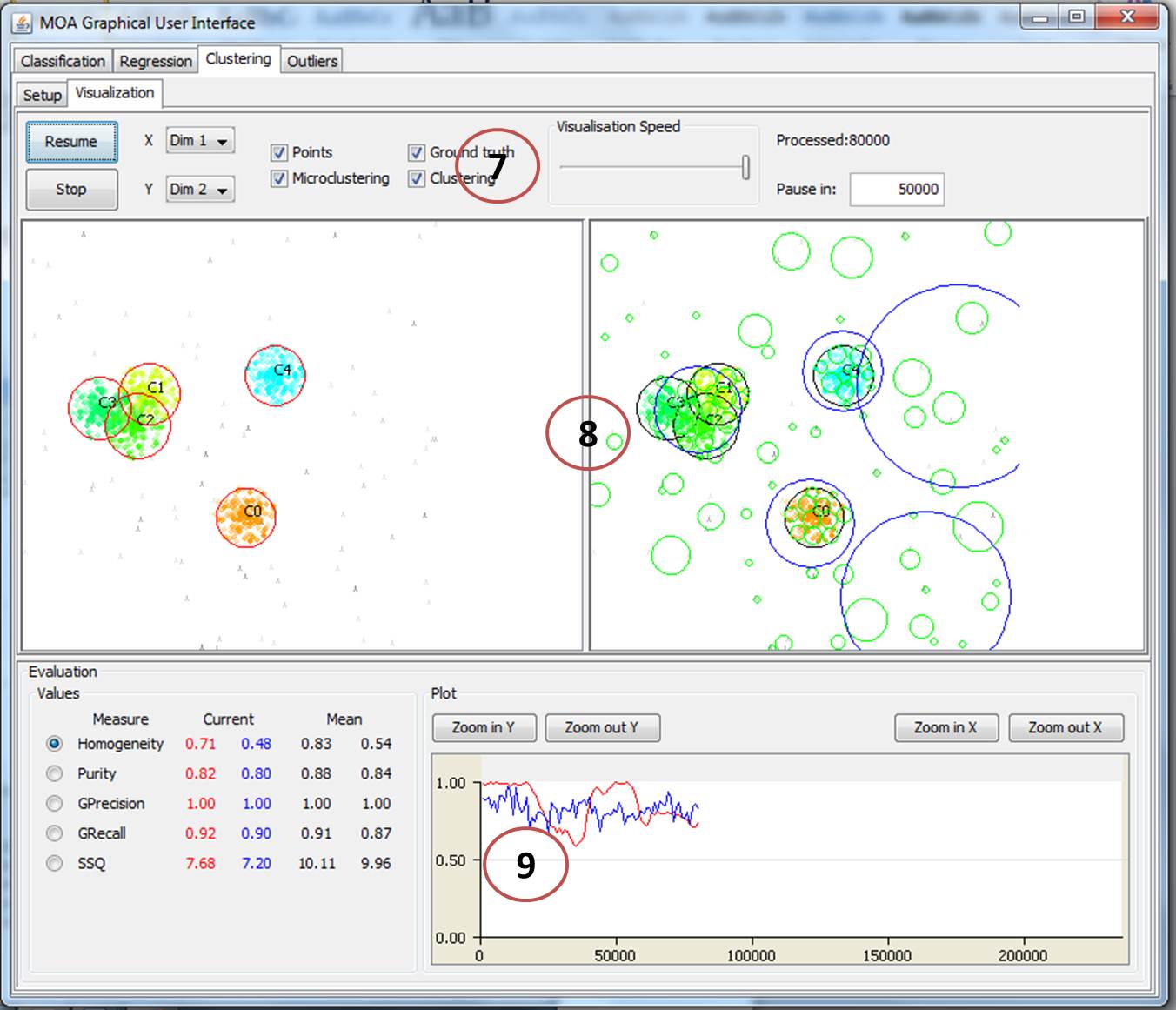
This part of the GUI allows to visually observe the clusters being built in real time, to observe performance metrics in real time and to interrupt and resume the clustering task. Here you can use the following GUI elements:

• Element 7 This part of the GUI provides buttons to start, stop (cancel) or to resume the cluster analysis. The cluster analysis usually stops after a user defined number of incoming data items is reached. Again, this can be specified in this element on the right hand side (in the screenshot this is set to 50,000 data items observed. Here you can also select if you want to display the micro-clusters, the actual clusters, the data points in the current time horizon, or/and the ground truth (the real clusters).
• Element 8 Displays for both cluster algorithms selected the micro-clusters, the actual clusters, the data points in the current time horizon, or/and the ground truth (the real clusters). “Algorithm 1″ is visualised on the left and “Algorithm 2″ is visualised on the right.
• Element 9 The performance metrics previously chosen in Element 4 are listed together with their current value on the left; and are plotted on the right in real time. You can only plot one metric at the same time. The blue plot is the metric for the algorithm visualised on the right hand side of element 8 (corresponds to Algorithm 2); and the red plot is the metric for the algorithm visualised on the left hand side of element 8 (corresponds to Algorithm 1).

Cluster evaluation methods implemented in MOA

• Extrinsic methods: Apply when the ground truth is available. The aim is to assign a score to the clustering when the ground truth is available.
  • Purity It is defined as:

    

    

    The higher the better, c is the number of clusters.

  • SSQ The sum of squared distances of the data items to their cluster centres. The smaller this is the better. Similar to Cohesion. The lower the better.
  • Homogeneity Each cluster contains only members of a single class. The lower bound is 0.0 and the upper bound is 1.0 (higher is better).
  • Completeness All members of a given class are assigned to the same cluster. The lower bound is 0.0 and the upper bound is 1.0 (higher is better).
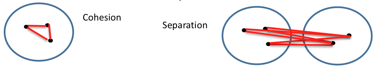
• Intrinsic methods: Apply when the ground truth is not available. Most of the time we would like to evaluate how compact and well separated the clusters are.
  • Silhouette Coefficient Is a combination of Separation and Cohesion measures.

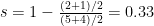
    Silhouette Coefficient s can be calculated for individual points, as well as clusters. For an individual point, a = average distance of i to the points in the same cluster; b = average distance of i to points in another cluster.

    

    This is typically a value between 0 and 1 assuming that a<b. The closer this is to 1 the better.

    

    In this example:

    

    In MOA the average silhouette is calculated for a set of clusters.

  Task 2: Data Stream Clustering Configuration

  First you need to configure your evolving data stream. Click in Element 3 on the edit button for the data stream. This will open the following dialog:

  

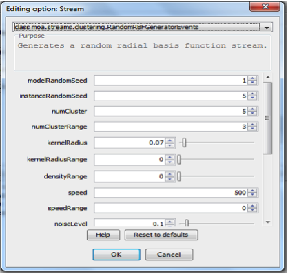
  On the top of the dialog you can select either to load your own stream data from an ARFF formatted file, or you can select the RandomRBFGeneratorEvents stream. This is a stream that constantly evolves and changes the position of the true clusters. Accept the settings as they are. We will revisit some of the settings a little later. Next click on the edit button for Algorithm 1, to set the first data stream clustering algorithm. A new dialog should open. On the top of this dialog, you can select the cluster algorithm. Please select Clustream.

  The dialog should now display the settings for Clustream as shown in the following figure:

  

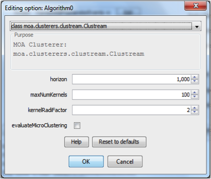
  With the horizon you can specify the time horizon for the macro cluster calculation. Here macro-clusters would be generated every 1000 data elements received. The setting maxNumOfKernels specifies the number of micro-clusters, and with the setting kernelRadiFactor you can take influence on the radius (boundary) of a micro-cluster (i.e. increase or decrease the boundaries). Keep the default settings. Next configure Algorithm 2 the same way. Select some evaluation metrics in element 4, in particular select SSQ. Click on the “Visualisation” tab in element 2, next click start (in element 7) and observe the clusters being generated and updated in real time. Play around with the selections in element 7, you can stop and resume the algorithm execution any time by using the controls in element 7.

  Exercises

  Exercise 1 Try to figure out how the different aspects of the cluster algorithm are visualised:

  Briefly note down how micro-clusters are visualised:

  Briefly note down how actual clusters are visualised:

  Briefly note down how the ground truth is visualised:

  Now play around with the evaluation metrics, please note that there are many more metrics then the ones we have learned about in this tutorial.

  Task 3: Fine tuning your Clustream algorithm

  The RandomRBFGeneratorEvents stream you used in Task 1 is constantly evolving, which can be managed by two parameters in the stream dialog. The parameter speed moves the real cluster centres by a predefined distance of 0.01 every X points, and the parameter speedRange, which is the
  Speed/Velocity point offset.

  Exercise 2 Double the speed to 1000 and set speedRange to 10. Also increase the noise level to 0.333, which means that about every third data item is randomly generated.

  Now try to find settings that keep the SSQ metric low. Note down your observations, i.e. what changes do you observe when you increase the number of micro-clusters, or when you change the radius:

  Task 4: Compare two data stream algorithms

  Exercise 3 Now use the same settings for the data stream as you used in Task 2, and set CluStream as Algorithm 1 with the same settings that have achieved the best result in Task 2. But this time you use for “Algorithm 2″ Clustree. This is a hierarchical clustering algorithm and allows adjusting two parameters, the horizon and the height of the hierarchy. Try to optimise the settings for Clustree. Again note down your observations:

  Task 5: Experiment

  Exercise 4 Experiment with other clustering algorithms and see if you can find an algorithm with a setting that outperforms Clustream and Clustree on the data stream setting outlined in Task 2.

  You may also examine the impact of changes in the data to the algorithms, i.e. increase the level of noise and observe which algorithms copes best with these changes.