Getting Started
This tutorial is a basic introduction to MOA. Massive Online Analysis (MOA) is a software environment for implementing algorithms and running experiments for online learning from evolving data streams. We suppose that MOA is installed in your system, if not, you can download MOA from here.
Start a graphical user interface for configuring and running tasks with the command:
java -cp moa.jar -javaagent:sizeofag-1.0.0.jar moa.gui.GUI
or using the script
bin/moa.sh
or
bin/moa.bat
Click ’Configure’ to set up a task, when ready click to launch a task click ’Run’. Several tasks can be run concurrently. Click on different tasks in the list and control them using the buttons below. If textual output of a task is available it will be displayed in the middle of the GUI, and can be saved to disk.
Note that the command line text box displayed at the top of the window represents textual commands that can be used to run tasks on the command line. The text can be selected then copied onto the clipboard. In the bottom of the GUI there is a graphical display of the results. It is possible to compare the results of two different tasks: the current task is displayed in red, and the selected previously is in blue.
The Classification Graphical User Interface
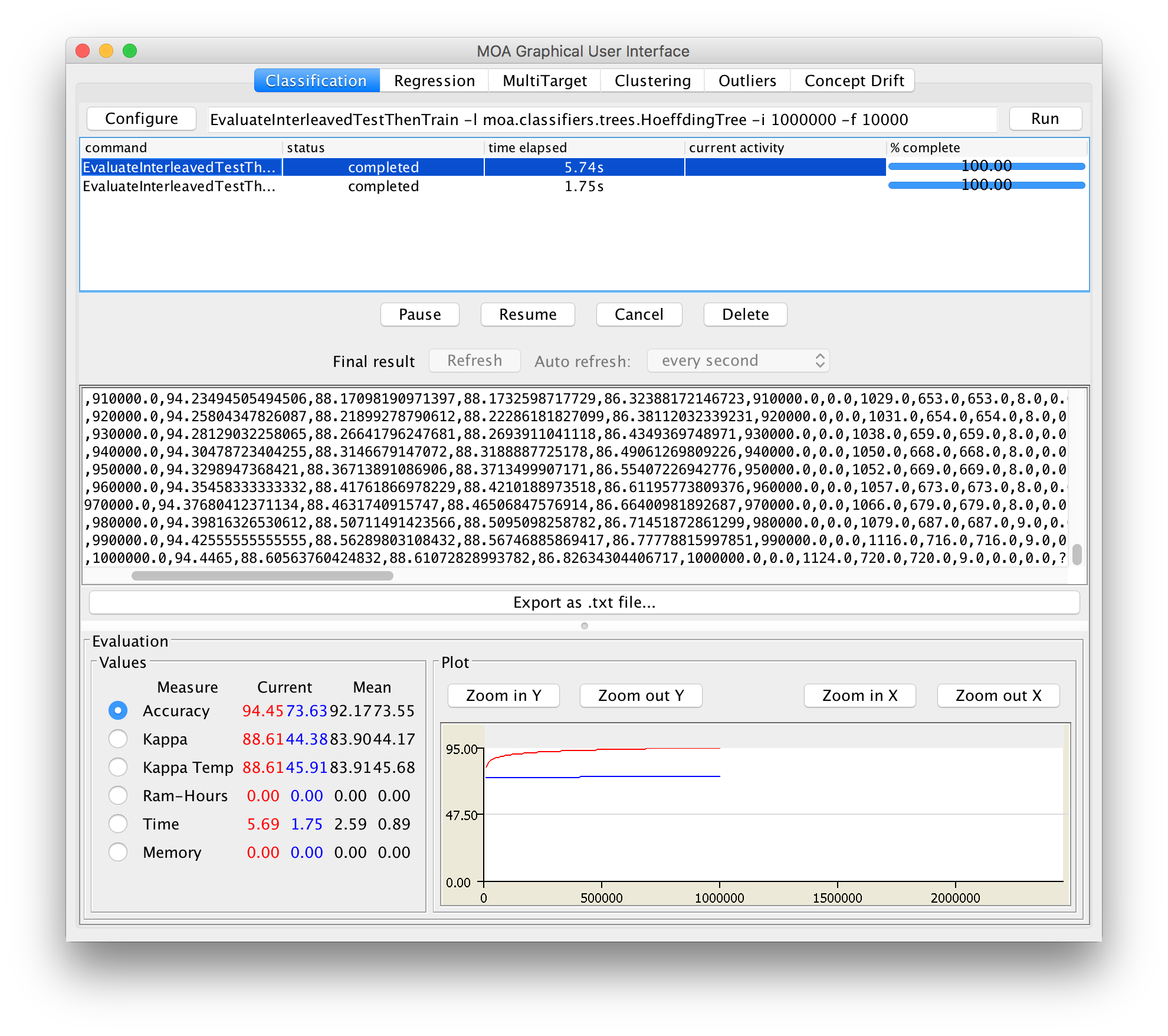
We start comparing the accuracy of two classifiers. First, we explain briefly two different data stream evaluations.
Data streams Evaluation
The most significant requirements for a data stream setting are the following:
- Requirement 1 Process an example at a time, and inspect it only once (at most)
- Requirement 2 Use a limited amount of memory
- Requirement 3 Work in a limited amount of time
- Requirement 4 Be ready to predict at any time
These requirements fit in a repeating cycle:

- The algorithm is passed the next available example from the stream (requirement 1).
- The algorithm processes the example, updating its data structures. It does so without exceeding the memory bounds set on it (requirement 2), and as quickly as possible (requirement 3).
- The algorithm is ready to accept the next example. On request it is able to predict the class of unseen examples (requirement 4).
In traditional batch learning the problem of limited data is overcome by analyzing and averaging multiple models produced with different random arrangements of training and test data. In the stream setting the problem of (effectively) unlimited data poses different challenges. One solution involves taking snapshots at different times during the induction of a model to see how much the model improves. When considering what procedure to use in the data stream setting, one of the unique concerns is how to build a picture of accuracy over time. Two main approaches arise:
- Holdout: When traditional batch learning reaches a scale where crossvalidation is too time consuming, it is often accepted to instead measure performance on a single holdout set. This is most useful when the division between train and test sets have been pre-defined, so
that results from different studies can be directly compared. - Interleaved Test-Then-Train or Prequential: Each individual example can be used to test the model before it is used for training, and from this the accuracy can be incrementally updated. When intentionally performed in this order, the model is always being tested on examples it has not seen. This scheme has the advantage that no holdout set is needed for testing, making maximum use of the available data. It also ensures a smooth plot of accuracy over time, as each individual example will become increasingly less significant to the overall average.
Holdout evaluation gives a more accurate estimation of the accuracy of the classifier on more recent data. However, it requires recent test data that it is difficult to obtain for real datasets. Gama et al. propose to use a forgetting mechanism for estimating holdout accuracy using prequential accuracy: a sliding window of size w with the most recent observations, or fading factors that weigh observations using a decay factor alpha. The output of the two mechanisms is very similar (every window of size w0 may be approximated by some decay factor alpha0). As data stream classification is a relatively new field, such evaluation practices are not nearly as well researched and established as they are in the traditional batch setting.
Exercises
To familiarize yourself with the functions discussed so far, please do the following two exercises. The solutions to these and other exercises in this tutorial are given at the end.
Exercise 1 Compare the accuracy of the Hoeffding Tree with the Naive Bayes classifier, for a RandomTreeGenerator stream of 1,000,000 instances using Interleaved Test-Then-Train evaluation. Use for all exercises a sample frequency of 10,000.
Exercise 2 Compare and discuss the accuracy for the same stream of the previous exercise using three different evaluations with a Hoeffding Tree:
- Periodic Held Out with 1,000 instances for testing
- Interleaved Test Then Train
- Prequential with a sliding window of 1,000 instances.
Drift Stream Generators
MOA streams are build using generators, reading ARFF files, joining several streams, or filtering streams. MOA streams generators allow to simulate potentially infinite sequence of data. Two streams evolving on time are:
- Rotating Hyperplane
- Random RBF Generator
To model concept drift we only have to set up the drift parameter of the stream.
Exercises
Exercise 3 Compare the accuracy of the Hoeffding Tree with the Naive Bayes classifier, for a RandomRBFGeneratorDrift stream of 1,000,000 instances with speed change of 0,001 using Interleaved Test-Then-Train evaluation.
Exercise 4 Compare the accuracy for the same stream of the previous exercise using three different classifiers:
- Hoeffding Tree with Majority Class at the leaves
- Hoeffding Adaptive Tree
- OzaBagAdwin with 10 HoeffdingTree
Using the command line
An easy way to use the command line, is to copy and paste the text in the Configuration line of the Graphical User Interface. For example, suppose we want to process the task
EvaluatePrequential -l trees.HoeffdingTree -i 1000000 -w 10000
using the command line. We simply write
java -cp moa.jar -javaagent:sizeofag-1.0.0.jar moa.DoTask \
"EvaluatePrequential -l trees.HoeffdingTree -i 1000000 \
-e (WindowClassificationPerformanceEvaluator -w 10000)"
Note that some parameters are missing, since they use default values.
Learning and Evaluating Models
The moa.DoTask class is the main class for running tasks on the command line. It will accept the name of a task followed by any appropriate parameters. The first task used is the LearnModel task. The -l parameter specifies the learner, in this case the HoeffdingTree class. The -s parameter specifies the stream to learn from, in this case generators.WaveformGenerator is specified, which is a data stream generator that produces a three-class learning problem of identifying three types of waveform. The -m option specifies the maximum number of examples to train the learner with, in this case one million examples. The -O option specifies a file to output the resulting model to:
java -cp moa.jar -javaagent:sizeofag-1.0.0.jar moa.DoTask \
LearnModel -l trees.HoeffdingTree \
-s generators.WaveformGenerator -m 1000000 -O model1.moa
This will create a file named model1.moa that contains the decision stump model that was induced during training. The next example will evaluate the model to see how accurate it is on a set of examples that are generated using a different random seed. The EvaluateModel task is given the parameters needed to load the model produced in the previous step, generate a new waveform stream with a random seed of 2, and test on one million examples:
java -cp moa.jar -javaagent:sizeofag-1.0.0.jar moa.DoTask \
"EvaluateModel -m file:model1.moa \
-s (generators.WaveformGenerator -i 2) -i 1000000"
This is the first example of nesting parameters using brackets. Quotes have been added around the description of the task, otherwise the operating system may be confused about the meaning of the brackets. After evaluation the following statistics are output:
classified instances = 1,000,000
classifications correct (percent) = 84.474
Kappa Statistic (percent) = 76.711
Note the the above two steps can be achieved by rolling them into one, avoiding the need to create an external file, as follows:
java -cp moa.jar -javaagent:sizeofag-1.0.0.jar moa.DoTask \
"EvaluateModel -m (LearnModel -l trees.HoeffdingTree \
-s generators.WaveformGenerator -m 1000000) \
-s (generators.WaveformGenerator -i 2) -i 1000000"
The task EvaluatePeriodicHeldOutTest will train a model while taking snapshots of performance using a held-out test set at periodic intervals. The following command creates a comma separated values file, training the HoeffdingTree classifier on the WaveformGenerator data, using the first 100 thousand examples for testing, training on a total of 100 million examples, and testing every one million examples:
java -cp moa.jar -javaagent:sizeofag-1.0.0.jar moa.DoTask \
"EvaluatePeriodicHeldOutTest -l trees.HoeffdingTree \
-s generators.WaveformGenerator \
-n 100000 -i 10000000 -f 1000000" > dsresult.csv
Exercises
Exercise 5 Repeat the experiments of exercises 1 and 2 using the command line.
Exercise 6 Compare accuracy and RAM-Hours needed using a prequential evaluation (sliding window of 1,000 instances) of 1,000,000 instances for a Random Radius Based Function stream with speed of change 0,001 using the following methods:
- OzaBag with 10 HoeffdingTree
- OzaBagAdwin with 10 HoeffdingTree
- LeveragingBag with 10 HoeffdingTree
Regression
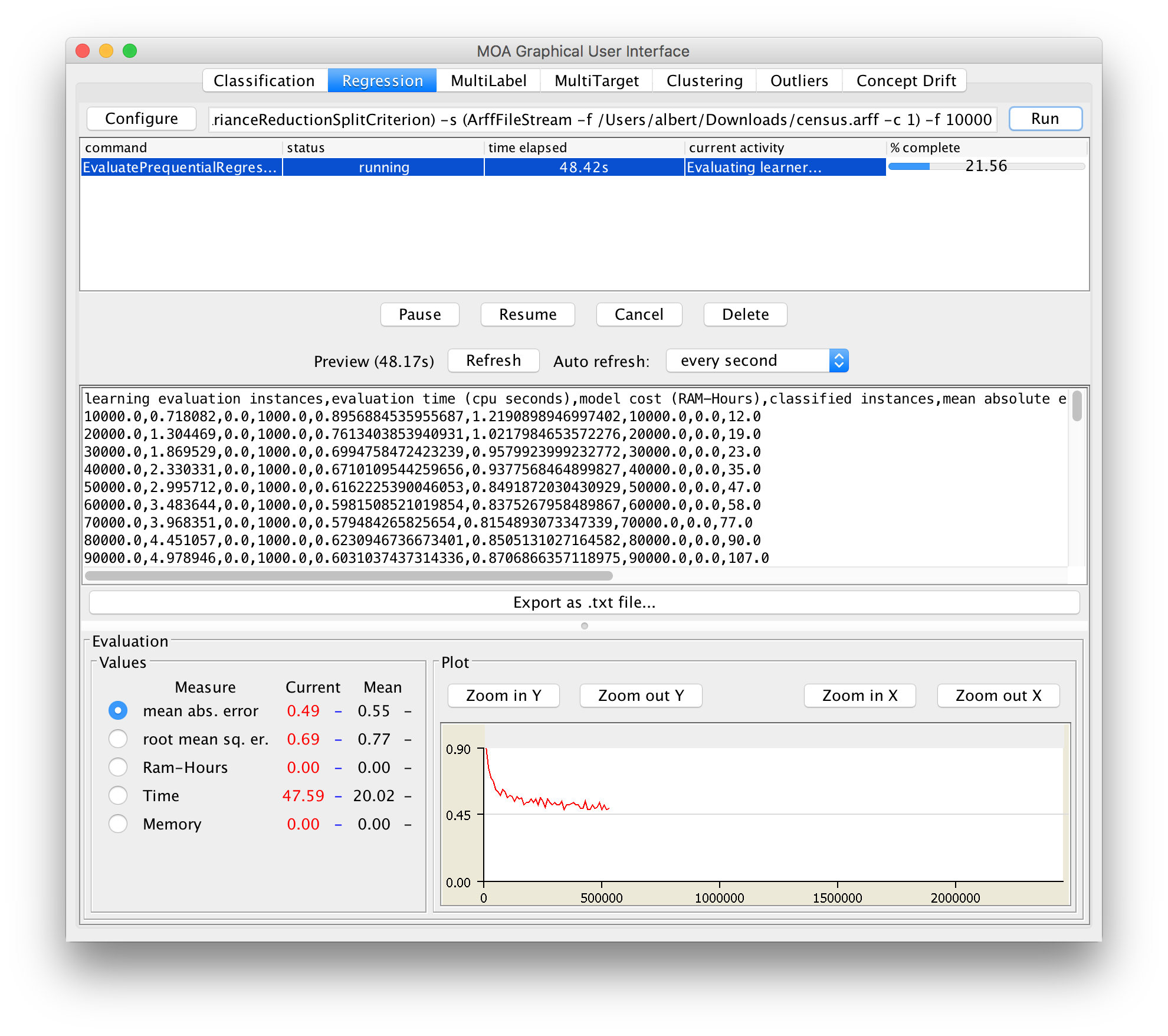
For regression, let’s go back to the GUI. Select the Regression tab. Click ”Configure” and explore the options. You will see that there is a lot less choice than for classification. This is not necessarily a problem, because algorithms like the tree-based FIMTDD method work really well in practise. Run the default configuration for a first exploration of the regression tab. As we are abusing a classification dataset here, as generated by the RandomTreeGenerator, it should come as no surprise that the results are not that convincing. For a better experience, go back to the configuration, and select ArffFileStream as the stream source, and provide some large numeric arff file. You could use the ”census.arff” file and specify the first attribute as the target: -c 1. Now run FIMTDD again. If you want a faster regressor, also try the Perceptron. For better results, but slower execution, experiment with the various (random) rule learners.
Tutorial 2 and Tutorial 3
Answers To Exercises
- Naive Bayes: 73:63% Hoeffding Tree : 94:45%
- Periodic Held Out with 1,000 instances for testing :96:5%
Interleaved Test Then Train : 94:45%
Prequential with a sliding window of 1,000 instances: 96:7%. - Naive Bayes: 53:14% Hoeffding Tree : 57:60%
- Hoeffding Tree with Majority Class at Leaves: 51:71%
Hoeffding Adaptive Tree: 66:26%
OzaBagAdwin with 10 HoeffdingTree: 68:11% - EvaluateInterleavedTestThenTrain -i 1000000
EvaluateInterleavedTestThenTrain -l trees.HoeffdingTree -i 1000000
EvaluatePeriodicHeldOutTest -n 1000 -i 1000000
EvaluateInterleavedTestThenTrain -l trees.HoeffdingTree -i 1000000
EvaluatePrequential -l trees.HoeffdingTree -i 1000000 - OzaBag with 10 HoeffdingTree:
- 62.1% Accuracy, 4×10⁻⁴ RAM-Hours
OzaBagAdwin with 10 HoeffdingTree:
- 71:5% Accuracy, 2:93×10-6 RAM-Hours
LeveragingBag with 10 HoeffdingTree:
- 84.40% Accuracy, 1:25x 10-4 RAM-Hours